
| 일 | 월 | 화 | 수 | 목 | 금 | 토 |
|---|---|---|---|---|---|---|
| 1 | ||||||
| 2 | 3 | 4 | 5 | 6 | 7 | 8 |
| 9 | 10 | 11 | 12 | 13 | 14 | 15 |
| 16 | 17 | 18 | 19 | 20 | 21 | 22 |
| 23 | 24 | 25 | 26 | 27 | 28 | 29 |
| 30 |
- 파이썬
- Machine Learning Advanced
- 코딩테스트
- eda
- 튜토리얼
- Python
- Image Segmentation
- TEAM EDA
- 협업필터링
- 알고리즘
- DilatedNet
- Segmentation
- 큐
- Object Detection
- 입문
- 3줄 논문
- hackerrank
- 나는 리뷰어다
- 엘리스
- 스택
- TEAM-EDA
- pytorch
- DFS
- 나는리뷰어다
- 한빛미디어
- 추천시스템
- Recsys-KR
- Semantic Segmentation
- 프로그래머스
- MySQL
- Today
- Total
TEAM EDA
[파이토치로 시작하는 딥러닝 기초] 2.4 Weight initialization 본문
이번 글에서는 PyTorch로 Weight Initialization 하는 것에 대해서 배워보도록 하겠습니다. 이번 글은 EDWITH에서 진행하는 파이토치로 시작하는 딥러닝 기초를 토대로 하였고 같이 스터디하는 팀원분들의 자료를 바탕으로 작성하였습니다.
목차
- Why good initialization?
- RBM / DBN
- Xavier / He initialization
- Code : mnist_nn_xavier
1. Why good initialization?

weight 초기화와 관련해서 연구한 내용을 보면, weight 초기화 방법을 적용한 ~ N이 다른 모델에 비해 학습속도와 에러 모두 낮은 것을 볼 수 있습니다. 그렇다면 어떤 식으로 초기화를 할 수 있을까요?

- 가중치 초기값이 0이거나 동일한 경우
- 모든 뉴런이 동일한 출력값을 내보내므로 역전파시에 동일한 그래디언트 값을 가지며 학습이 잘 안됨
- 난수인 경우 (Uniform, Normal Distribution)
- 가중치 초기값이 크면 그래디언트 소실이나 폭주가 발생 -> 작은 값으로 초기화
- 신경망이 깊어질 수록 모든 출력이 0이 되는 문제가 발생하거나 vanishing gradient 발생
- Restricted Boltzmann Machine (RBM)
2. RBM / DBN(Deep Belief Network)

위의 모습을 RBM이라고 하는데, 같은 layer의 weight 끼리는 연결이 없고(Restricted) 다른 layer의 node와는 모두 연결이 된 것을 의미합니다. 이 머신이 하는 일은 입력 X가 들어오면 Y를 뱉는 Encoding와 Y가 들어오면 X'을 뱉는 Decoding을 합니다. 그렇다면, RBM으로 어떻게 가중치 초기화를 할 수 있을까요?
Hinton 교수님은 여기에 pre-training step이라는 것을 제안합니다. 왼쪽을 보면 한단계씩 진행하게 되는데,

- (a) : RBM을 통해서 입력 x가 주어질 때, Y가 무엇이 나오는 지 계산. (w1 : x와 h1간의 weight)
- (b) : w1은 고정시킨 상태로 h1과 h2간의 RBM을 진행
- (c) : 마지막 layer h3와 h2간의 RBM을 진행
- Fine-tuning : RBM으로 학습된 weight들에 일반적으로 사용하는 neural network 학습 방식을 적용시켜서 weight를 업데이트하는 것을 의미
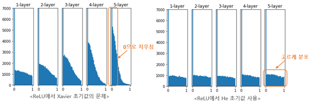
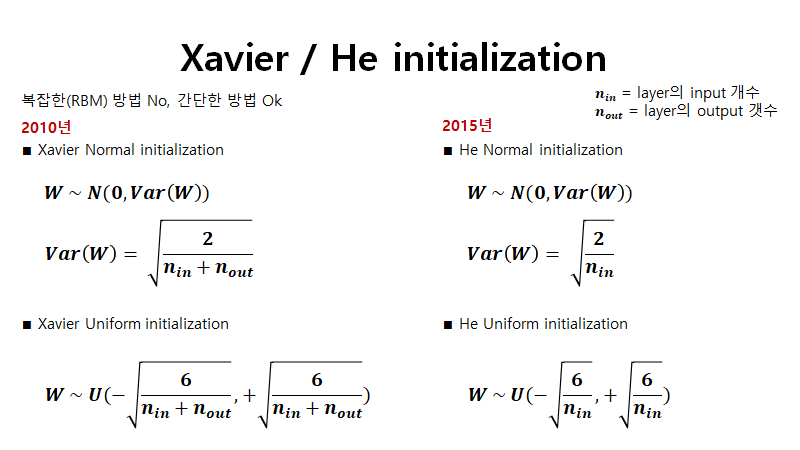
3. Xavier / He initialization
기존의 무작위 수로 초기화와 다르게 Layer의 특성에 맞춰서 초기화하는 방법. Xavier의 경우 기존보다 좋은 성능을 보이지만 ReLU에서 출력 값이 0으로 수렴하는 문제가 종종 발생하였고 이를 해결하기 위해 나온 방법이 He initialization입니다.
4. Code : mnist_nn_xavier
# xavier initialization
torch.nn.init.xavier_uniform_(linear1.weight)
torch.nn.init.xavier_uniform_(linear2.weight)
torch.nn.init.xavier_uniform_(linear3.weight)
# Lab 10 MNIST and softmax
import torch
import torchvision.datasets as dsets
import torchvision.transforms as transforms
import random
device = 'cuda' if torch.cuda.is_available() else 'cpu'
# for reproducibility
random.seed(777)
torch.manual_seed(777)
if device == 'cuda':
torch.cuda.manual_seed_all(777)
# parameters
learning_rate = 0.001
training_epochs = 15
batch_size = 100
# MNIST dataset
mnist_train = dsets.MNIST(root='MNIST_data/',
train=True,
transform=transforms.ToTensor(),
download=True)
mnist_test = dsets.MNIST(root='MNIST_data/',
train=False,
transform=transforms.ToTensor(),
download=True)
# dataset loader
data_loader = torch.utils.data.DataLoader(dataset=mnist_train,
batch_size=batch_size,
shuffle=True,
drop_last=True)
# nn layers
linear1 = torch.nn.Linear(784, 256, bias=True)
linear2 = torch.nn.Linear(256, 256, bias=True)
linear3 = torch.nn.Linear(256, 10, bias=True)
relu = torch.nn.ReLU()
# xavier initialization
torch.nn.init.xavier_uniform_(linear1.weight)
torch.nn.init.xavier_uniform_(linear2.weight)
torch.nn.init.xavier_uniform_(linear3.weight)
# model
model = torch.nn.Sequential(linear1, relu, linear2, relu, linear3).to(device)
# define cost/loss & optimizer
criterion = torch.nn.CrossEntropyLoss().to(device) # Softmax is internally computed.
optimizer = torch.optim.Adam(model.parameters(), lr=learning_rate)
total_batch = len(data_loader)
for epoch in range(training_epochs):
avg_cost = 0
for X, Y in data_loader:
# reshape input image into [batch_size by 784]
# label is not one-hot encoded
X = X.view(-1, 28 * 28).to(device)
Y = Y.to(device)
optimizer.zero_grad()
hypothesis = model(X)
cost = criterion(hypothesis, Y)
cost.backward()
optimizer.step()
avg_cost += cost / total_batch
print('Epoch:', '%04d' % (epoch + 1), 'cost =', '{:.9f}'.format(avg_cost))
print('Learning finished')
# Test the model using test sets
with torch.no_grad():
X_test = mnist_test.test_data.view(-1, 28 * 28).float().to(device)
Y_test = mnist_test.test_labels.to(device)
prediction = model(X_test)
correct_prediction = torch.argmax(prediction, 1) == Y_test
accuracy = correct_prediction.float().mean()
print('Accuracy:', accuracy.item())
# Get one and predict
r = random.randint(0, len(mnist_test) - 1)
X_single_data = mnist_test.test_data[r:r + 1].view(-1, 28 * 28).float().to(device)
Y_single_data = mnist_test.test_labels[r:r + 1].to(device)
print('Label: ', Y_single_data.item())
single_prediction = model(X_single_data)
print('Prediction: ', torch.argmax(single_prediction, 1).item())
참고자료
'EDA Study > PyTorch' 카테고리의 다른 글
| [파이토치로 시작하는 딥러닝 기초] 2.6 Batch Normalization (0) | 2020.03.20 |
|---|---|
| [파이토치로 시작하는 딥러닝 기초] 2.5 Dropout (0) | 2020.03.20 |
| [파이토치로 시작하는 딥러닝 기초] 2.3 ReLU (0) | 2020.03.20 |
| [파이토치로 시작하는 딥러닝 기초] 2.1~2 Perceptron, Multi Layer Perceptron (0) | 2020.03.20 |
| [파이토치로 시작하는 딥러닝 기초] 1.6 Softmax Classification (0) | 2020.03.20 |


