
| 일 | 월 | 화 | 수 | 목 | 금 | 토 |
|---|---|---|---|---|---|---|
| 1 | 2 | 3 | 4 | 5 | 6 | |
| 7 | 8 | 9 | 10 | 11 | 12 | 13 |
| 14 | 15 | 16 | 17 | 18 | 19 | 20 |
| 21 | 22 | 23 | 24 | 25 | 26 | 27 |
| 28 | 29 | 30 | 31 |
- 한빛미디어
- 입문
- 큐
- Machine Learning Advanced
- 튜토리얼
- Image Segmentation
- 협업필터링
- MySQL
- 나는리뷰어다
- Segmentation
- 3줄 논문
- eda
- 프로그래머스
- 나는 리뷰어다
- hackerrank
- DilatedNet
- DFS
- TEAM-EDA
- 파이썬
- Python
- 알고리즘
- Recsys-KR
- 추천시스템
- 스택
- TEAM EDA
- 코딩테스트
- 엘리스
- pytorch
- Object Detection
- Semantic Segmentation
- Today
- Total
TEAM EDA
kaggle - Rossmann Store sales Prediction (1) 본문
kaggle - Rossmann Store sales Prediction (1)
김현우 2019. 9. 10. 12:53
Author: Team-EDA 김현우,박주연,이주영,이지예,주진영,홍정아
NOTE : 아래의 자료는 Christian Thieli의 자료를 토대로 스터디원이 함께 배운 내용과 IDEA를 추가해서 만든 자료입니다. 첫번째 자료에서는 Vote가 가장높은 자료를 토대로 팀원들의 아이디어를 합쳐서 데이터 탐색을 진행하고, 두번째 자료에서는 다른사람들의 EDA자료를 통해서 아이디어를 더 발굴할 것 입니다. 마지막으로는 얻을 아이디어를 통해서 모델링을 하도록 하겠습니다.
1. 대회 소개 ( Introduction )
2.데이터 설명 ( Data Description )
3.패키지 설치 및 불러오기 ( Retrieving the Data )
4.데이터 구조 확인 ( Data Structure )
5.데이터 전처리 ( Data Preparation )
6.탐색적 데이터 분석( Data Exploration )
6.1 Open의 NA값 (NA's Open of store 622)
6.2 Test와 Train의 unique한 데이터의 갯수가 다름
6.3 Train sales의 분석
6.4 그 외 변수간의 분석
6.5 store.csv의 분석
7.추가사항
1. 대회소개
Competition Description
Rossmann은 7개의 유럽 국가에서 3,000개가 넘는 약국을 운영하고 있습니다. 현재 Rossmann 매장 관리자는 최대 6주 전부터 일일 판매량을 예측해야합니다. 상점 판매는 판촉, 경쟁, 학교 및 공휴일, 계절 및 지역 등 많은 요인의 영향을받습니다. 고유 한 상황에 따라 수천 명의 개별 관리자가 판매를 예측하면 결과의 정확성이 상당히 달라질 수 있습니다.
첫 번째 Kaggle 경쟁에서, Rossmann은 독일 전역에있는 1,115 개 매장에 대한 6주 일일 판매량을 예측하는 대회를 진행하려고 합니다. 신뢰할 수있는 판매 예측을 통해 매장 관리자는 효과적인 직원 일정을 만들어 생산성과 동기를 높일 수 있습니다. 당신이 강력한 예측 모델을 만들도록 도와줌으로써 매장 관리자는 고객과 팀에게 가장 중요한 것에 집중할 수 있습니다 !!!
Evaluation
제출파일은 RMSE로 계산되고 RMSE는 아래와 같이 계산됩니다.
$$$ RMSPE= \sqrt{ \frac{1}{n}\sum_{i=1}^n (\frac{y_i - \widehat{y_i}}{y_i})^2} $$$
where y_i denotes the sales of a single store on a single day and yhat_i denotes the corresponding prediction. Any day and store with 0 sales is ignored in scoring.
여기서 y_i는 하루에 단일 상점의 판매를 나타내고 yhat_i는 해당 예측을 나타냅니다. 판매량이 0인 상점이나 날짜의 경우 무시됩니다.
2. 데이터설명
Data Description
1,115 Rossmann 상점에 대한 과거 판매 데이터가 제공됩니다. 이 작업은 테스트 세트의 "판매"열을 예측하는 것입니다. 데이터 세트의 일부 상점은 개장을 위해 일시적으로 폐쇄되었습니다.
Files
- train.csv - historical data including Sales
- test.csv - historical data excluding Sales
- sample_submission.csv - a sample submission file in the correct format
- store.csv - supplemental information about the stores
Data fields
Most of the fields are self-explanatory. The following are descriptions for those that aren't.
Id- an Id that represents a (Store, Date) duple within the test setStore- a unique Id for each storeSales- the turnover for any given day (this is what you are predicting)Customers- the number of customers on a given dayOpen- an indicator for whether the store was open: 0 = closed, 1 = openStateHoliday- indicates a state holiday. Normally all stores, with few exceptions, are closed on state holidays. Note that all schools are closed on public holidays and weekends. a = public holiday, b = Easter holiday, c = Christmas, 0 = NoneSchoolHoliday- indicates if the (Store, Date) was affected by the closure of public schoolsStoreType- differentiates between 4 different store models: a, b, c, dAssortment- describes an assortment level: a = basic, b = extra, c = extendedCompetitionDistance- distance in meters to the nearest competitor storeCompetitionOpenSince[Month/Year]- gives the approximate year and month of the time the nearest competitor was openedPromo- indicates whether a store is running a promo on that dayPromo2- Promo2 is a continuing and consecutive promotion for some stores: 0 = store is not participating, 1 = store is participatingPromo2Since[Year/Week]- describes the year and calendar week when the store started participating in Promo2PromoInterval- describes the consecutive intervals Promo2 is started, naming the months the promotion is started anew. E.g. "Feb,May,Aug,Nov" means each round starts in February, May, August, November of any given year for that store
3.패키지 설치 및 불러오기
먼저 필요로하는 패키지를 불러오도록 하겠습니다.
# loading packages
library(data.table)
library(zoo)
library(dplyr)
library(ggplot2)
library(forecast)
library(ggrepel)
# data loadings
test <- fread("../input/test.csv")
train <- fread("../input/train.csv")
store <- fread("../input/store.csv")> str(train)
#check data type of 1.Date (Date) 2.State Holiday,SchoolHoliday (categorical) 3.Store (store index)Classes ‘data.table’ and 'data.frame': 1017209 obs. of 9 variables:
$ Store : int 1 2 3 4 5 6 7 8 9 10 ...
$ DayOfWeek : int 5 5 5 5 5 5 5 5 5 5 ...
$ Date : chr "2015-07-31" "2015-07-31" "2015-07-31" "2015-07-31" ...
$ Sales : int 5263 6064 8314 13995 4822 5651 15344 8492 8565 7185 ...
$ Customers : int 555 625 821 1498 559 589 1414 833 687 681 ...
$ Open : int 1 1 1 1 1 1 1 1 1 1 ...
$ Promo : int 1 1 1 1 1 1 1 1 1 1 ...
$ StateHoliday : chr "0" "0" "0" "0" ...
$ SchoolHoliday: chr "1" "1" "1" "1" ...
- attr(*, ".internal.selfref")=<externalptr>> str(test) # Id(Submission) plus // Sales & customers Delete Classes ‘data.table’ and 'data.frame': 41088 obs. of 8 variables:
$ Id : int 1 2 3 4 5 6 7 8 9 10 ...
$ Store : int 1 3 7 8 9 10 11 12 13 14 ...
$ DayOfWeek : int 4 4 4 4 4 4 4 4 4 4 ...
$ Date : chr "2015-09-17" "2015-09-17" "2015-09-17" "2015-09-17" ...
$ Open : int 1 1 1 1 1 1 1 1 1 1 ...
$ Promo : int 1 1 1 1 1 1 1 1 1 1 ...
$ StateHoliday : chr "0" "0" "0" "0" ...
$ SchoolHoliday: chr "0" "0" "0" "0" ...
- attr(*, ".internal.selfref")=<externalptr># data type: str -> Date
train[, Date := as.Date(Date)] #(same code)train$Date <- as.Date(train$Date)
test[, Date := as.Date(Date)] #(same code)test$Date <- as.Date(test$Date)# reordered by Date
train <- train[order(Date)]
test <- test[order(Date)]summary(train) Store DayOfWeek Date Sales
Min. : 1.0 Min. :1.000 Min. :2013-01-01 Min. : 0
1st Qu.: 280.0 1st Qu.:2.000 1st Qu.:2013-08-17 1st Qu.: 3727
Median : 558.0 Median :4.000 Median :2014-04-02 Median : 5744
Mean : 558.4 Mean :3.998 Mean :2014-04-11 Mean : 5774
3rd Qu.: 838.0 3rd Qu.:6.000 3rd Qu.:2014-12-12 3rd Qu.: 7856
Max. :1115.0 Max. :7.000 Max. :2015-07-31 Max. :41551
Customers Open Promo StateHoliday
Min. : 0.0 Min. :0.0000 Min. :0.0000 Length:1017209
1st Qu.: 405.0 1st Qu.:1.0000 1st Qu.:0.0000 Class :character
Median : 609.0 Median :1.0000 Median :0.0000 Mode :character
Mean : 633.1 Mean :0.8301 Mean :0.3815
3rd Qu.: 837.0 3rd Qu.:1.0000 3rd Qu.:1.0000
Max. :7388.0 Max. :1.0000 Max. :1.0000
SchoolHoliday
Length:1017209
Class :character
Mode :character summary(test) #open of test havs 11 NA's / train open Mean 0.8301 vs test open Mean 0.8543 Id Store DayOfWeek Date
Min. : 1 Min. : 1.0 Min. :1.000 Min. :2015-08-01
1st Qu.:10273 1st Qu.: 279.8 1st Qu.:2.000 1st Qu.:2015-08-12
Median :20544 Median : 553.5 Median :4.000 Median :2015-08-24
Mean :20544 Mean : 555.9 Mean :3.979 Mean :2015-08-24
3rd Qu.:30816 3rd Qu.: 832.2 3rd Qu.:6.000 3rd Qu.:2015-09-05
Max. :41088 Max. :1115.0 Max. :7.000 Max. :2015-09-17
Open Promo StateHoliday SchoolHoliday
Min. :0.0000 Min. :0.0000 Length:41088 Length:41088
1st Qu.:1.0000 1st Qu.:0.0000 Class :character Class :character
Median :1.0000 Median :0.0000 Mode :character Mode :character
Mean :0.8543 Mean :0.3958
3rd Qu.:1.0000 3rd Qu.:1.0000
Max. :1.0000 Max. :1.0000
NA's :11 Train과 Test를 비교했을때, Test에 11개의 NA가 있는것을 확인할 수 있음. 이제부터 그에 대한 조사!!! check: 1. open mean이 좀 다른거, date 최소 최대
test[is.na(test$Open), ] # Only store 622| Id | Store | DayOfWeek | Date | Open | Promo | StateHoliday | SchoolHoliday |
|---|---|---|---|---|---|---|---|
| 10752 | 622 | 6 | 2015-09-05 | NA | 0 | 0 | 0 |
| 9040 | 622 | 1 | 2015-09-07 | NA | 0 | 0 | 0 |
| 8184 | 622 | 2 | 2015-09-08 | NA | 0 | 0 | 0 |
| 7328 | 622 | 3 | 2015-09-09 | NA | 0 | 0 | 0 |
| 6472 | 622 | 4 | 2015-09-10 | NA | 0 | 0 | 0 |
| 5616 | 622 | 5 | 2015-09-11 | NA | 0 | 0 | 0 |
| 4760 | 622 | 6 | 2015-09-12 | NA | 0 | 0 | 0 |
| 3048 | 622 | 1 | 2015-09-14 | NA | 1 | 0 | 0 |
| 2192 | 622 | 2 | 2015-09-15 | NA | 1 | 0 | 0 |
| 1336 | 622 | 3 | 2015-09-16 | NA | 1 | 0 | 0 |
| 480 | 622 | 4 | 2015-09-17 | NA | 1 | 0 | 0 |
2015-08-01 ~ 2015-09-17까지 Test data가 구성되어있음. 이 중 2015-09-05 ~ 2015-09-17까지의 Store 622의 data만 비어있다. 그 중 6일과 13일(7일 간격)은 일요일이라서 데이터 자체가 구성이 되지 않은 것 같다.
test %>% filter(Open %in% c("2015-09-06","2015-09-13")) # 역시나 데이터가 없는 걸 확인할 수 있음.| Id | Store | DayOfWeek | Date | Open | Promo | StateHoliday | SchoolHoliday |
|---|
<0 행> <또는 row.names의 길이가 0입니다>
이제
다른 store보고 채워넣을거예요.
-
2015-09-05 ~ 2015-09-17의 store 622를 제외한 다른 store의 open여부를 확인.
생각중) 근데 store가 같으니 promo도 동일한가?
생각중) 나라가 위에서 6개라는데 휴일은 다르지 않을까? -
store 622가 이유없이 open하지 않았던 과거가 있는 지 확인. ∵ 다른 곳이 열었음에도 store 622는 열지 않을 수 있으니깐.
Promo가 0일 때 이유 없이(다른 store가 안쉬는데) 쉬었던 경험이 많은지, 아닌지를 check.
생각중) 근처 Store(국가가 6개여서 나라마다 or 근처 위치마다를 check할 수 있으면 그것도 집어넣기.//Store.csv에 보면 competitor 정보도 주어져서 같이 확인하면 좋을 듯.)
생각중) Promo = 1이면 open 하지 않을까?
#1. 다른 store가 open 했는지 여부.
full <- bind_rows(train,test) # 아래로 추가시키는거.
full1 = full %>% filter(Date %in% c("2015-09-05","2015-09-07","2015-09-08","2015-09-09","2015-09-10","2015-09-11","2015-09-12","2015-09-14","2015-09-15","2015-09-16","2015-09-17"))
> table(full1$Open,full1$Date)
2015-09-05 2015-09-07 2015-09-08 2015-09-09 2015-09-10 2015-09-11 2015-09-12 2015-09-14 2015-09-15
0 0 1 1 1 0 1 2 3 3
1 855 854 854 854 855 854 853 852 852
2015-09-16 2015-09-17
0 3 3
1 852 852
# 대부분 open한것을 확인할 수 있음.생각중) Promo가 1이면 open 하는지에 대한 여부 확인.
# IDEA1: if Promo was 1, open also 1.
full_Promo <- full %>% filter(Promo==1)

ggplot(full_Promo, aes(x = Open, fill = factor(Promo))) +
  geom_bar(stat='count', position='dodge') +
  labs(x = 'Open') +
  geom_label(stat='count',aes(label=..count..), size=3) +
  scale_fill_manual("legend", values = c("pink")) +
  ggtitle("Promo is 1") +
  theme_gray()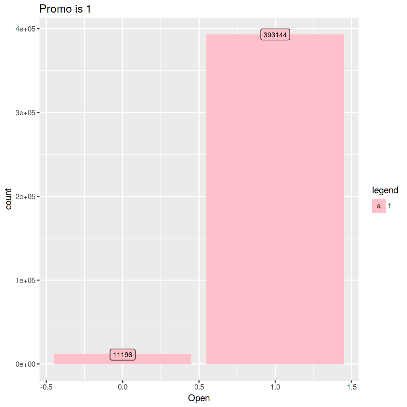
ggplot(full, aes(x = Open, fill = factor(Promo))) +
  geom_bar(stat='count', position='dodge') +
  labs(x = 'Open') +
  geom_label(stat='count',aes(label=..count..), size=3) +
  scale_fill_manual("legend", values = c("green","pink")) +
  ggtitle("Promo is 0(Green),Promo is 1(Pink)") +
  theme_gray()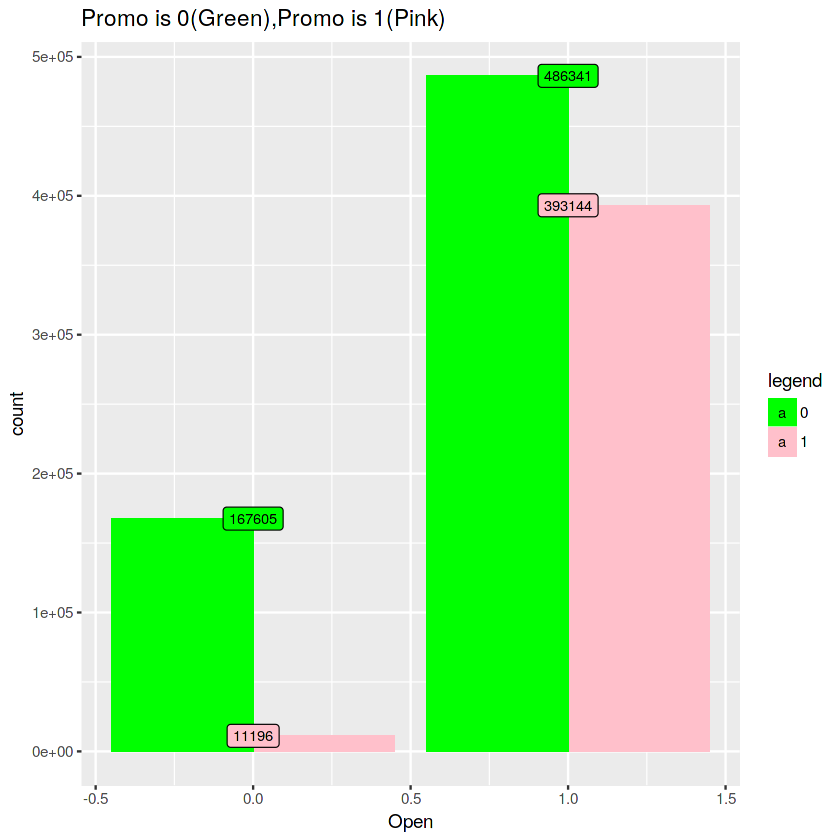
cat("\nProp Table\n")
prop.table(table(full_Promo$Promo,full_Promo$Open))
# 2.77 % -> open = 0 & promo = 1 why? 1. holiday (?) 2. not reason.
Prop Table
0 1
1 0.02768957 0.97231043# 1. check holiday
table(full$Date,full$Promo) # 그전에 promo가 동일 한지 부터 확인. 왜냐하면 국가가 6개니깐... 근데 중간에 데이터 손실이 있음. 1115 -> 935로 감소 -> 1115로 증가 -> 856로 증가(TEST) 0 1
2013-01-01 1114 0
2013-01-02 1115 0
2013-01-03 1115 0
2013-01-04 1115 0
2013-01-05 1115 0
2013-01-06 1115 0
2013-01-07 0 1115
2013-01-08 0 1115
.
.
.
2014-07-01 0 935
2014-07-02 0 935
2014-07-03 0 935
2014-07-04 0 935
2014-07-05 935 0
2014-07-06 935 0
2014-07-07 935 0
2014-07-08 935 0
2014-07-09 935 0
.
.
.
2014-12-31 935 0
2015-01-01 1115 0
.
.
.
2015-07-30 0 1115
2015-07-31 0 1115
2015-08-01 856 0
2015-08-02 856 0
.
.
.
2015-09-12 856 0
2015-09-13 856 0
2015-09-14 0 856
2015-09-15 0 856
2015-09-16 0 856
2015-09-17 0 856 table(full$Date,full$StateHoliday)
# 누구는 쉬는 날이고 누구는 쉬지 않는 날임. promo일 지라도 holiday이어서 쉴 가능성이 있음. 0 a b c
2013-01-01 0 1114 0 0
2013-01-02 1115 0 0 0
2013-01-03 1115 0 0 0
2013-01-04 1115 0 0 0
2013-01-05 1115 0 0 0
2013-01-06 806 309 0 0
2013-01-07 1115 0 0 0
.
.
.
2013-10-31 948 167 0 0
2013-11-01 536 579 0 0
.
.
.
2014-10-31 768 167 0 0
2014-11-01 536 399 0 0
.
.
.
table(full$Promo,full$StateHoliday)
# 11196 - 10796(7451+3345) = 400번 정도가 Promo 기간에 의미 없이 쉼.
0 a b c
0 633519 12989 3345 4100
1 393548 7451 3345 0#위에서 promo가 store마다 동일한 걸 확인했으니, promo면서 쉬는 놈들 조사.
full_promo1_open0 <- full %>% filter(Promo==1 & Open ==0)
nrow(full_promo1_open0)11196
full_promo1_open0[full_promo1_open0$Store==622,]
#우리의 target인 622는 promo일때도 쉬는 전과가 있음.
#3.1 알고보니 StateHoliday 상태여서 다 같이 쉰거 같음.| Store | DayOfWeek | Date | Sales | Customers | Open | Promo | StateHoliday | SchoolHoliday | Id | |
|---|---|---|---|---|---|---|---|---|---|---|
| 817 | 622 | 5 | 2013-03-29 | 0 | 0 | 0 | 1 | b | 1 | NA |
| 1986 | 622 | 3 | 2013-05-01 | 0 | 0 | 0 | 1 | a | 0 | NA |
| 4545 | 622 | 5 | 2014-04-18 | 0 | 0 | 0 | 1 | b | 1 | NA |
| 5642 | 622 | 4 | 2014-05-01 | 0 | 0 | 0 | 1 | a | 1 | NA |
| 7490 | 622 | 5 | 2014-10-03 | 0 | 0 | 0 | 1 | a | 0 | NA |
| 8880 | 622 | 5 | 2015-04-03 | 0 | 0 | 0 | 1 | b | 1 | NA |
| 9978 | 622 | 5 | 2015-05-01 | 0 | 0 | 0 | 1 | a | 0 | NA |
full_promo1_open0[full_promo1_open0$Date==c("2013-03-29","2013-05-01","2014-04-18","2014-05-01","2014-10-03","2015-04-03","2015-05-01"),] # 보면 다른 store 또한 쉼.
full %>% filter(Promo==1 & Open ==0)  %>% filter(StateHoliday == 0)  %>% nrow() # 위 400이랑 차이가난다. 무슨 실수를 한것일까 ??? 아 위에는 promo까지 더해준것이구나. promo가 0 일때 436개가 있지 않을까???

#궁금증3.2 StateHoliday 인데도 문열고 나온애 있을 수 있자나?
full %>% filter(StateHoliday != 0 & Open == 1) # 꽤 있는거 확인 가능. 그렇다면 우리의 622는?
full %>% filter(StateHoliday != 0 & Open == 1 & Store == 622) # 그런거 없음. 그리고 NA값은 어차피 stateholiday가 0이어서 의미 없었을 듯.

cat("Result: We can impute 1 when 2015.09.14~17") | Store | DayOfWeek | Date | Sales | Customers | Open | Promo | StateHoliday | SchoolHoliday | Id | |
|---|---|---|---|---|---|---|---|---|---|---|
| 211 | 6 | 5 | 2013-03-29 | 0 | 0 | 0 | 1 | b | 1 | NA |
| 218 | 13 | 5 | 2013-03-29 | 0 | 0 | 0 | 1 | b | 1 | NA |
| 225 | 20 | 5 | 2013-03-29 | 0 | 0 | 0 | 1 | b | 1 | NA |
| 232 | 27 | 5 | 2013-03-29 | 0 | 0 | 0 | 1 | b | 1 | NA |
| 211 | 6 | 5 | 2013-03-29 | 0 | 0 | 0 | 1 | b | 1 | NA |
| ... | ... | ... | ... | ... | ... | ... | ... | ... | ... | ... |
| ... | ... | ... | ... | ... | ... | ... | ... | ... | ... | ... |
| 10437 | 1087 | 5 | 2015-05-01 | 0 | 0 | 0 | 1 | a | 0 | NA |
| 10444 | 1094 | 5 | 2015-05-01 | 0 | 0 | 0 | 1 | a | 0 | NA |
| 10451 | 1102 | 5 | 2015-05-01 | 0 | 0 | 0 | 1 | a | 0 | NA |
| 10458 | 1109 | 5 | 2015-05-01 | 0 | 0 | 0 | 1 | a | 0 | NA |
836
| Store | DayOfWeek | Date | Sales | Customers | Open | Promo | StateHoliday | SchoolHoliday | Id |
|---|---|---|---|---|---|---|---|---|---|
| 85 | 2 | 2013-01-01 | 4220 | 619 | 1 | 0 | a | 1 | NA |
| 259 | 2 | 2013-01-01 | 6851 | 1444 | 1 | 0 | a | 1 | NA |
| 262 | 2 | 2013-01-01 | 17267 | 2875 | 1 | 0 | a | 1 | NA |
| 274 | 2 | 2013-01-01 | 3102 | 729 | 1 | 0 | a | 1 | NA |
| 335 | 2 | 2013-01-01 | 2401 | 482 | 1 | 0 | a | 1 | NA |
| ⋮ | ⋮ | ⋮ | ⋮ | ⋮ | ⋮ | ⋮ | ⋮ | ⋮ | ⋮ |
| 1019 | 6 | 2015-08-15 | NA | NA | 1 | 0 | a | 0 | 29031 |
| 1027 | 6 | 2015-08-15 | NA | NA | 1 | 0 | a | 0 | 29037 |
| 1056 | 6 | 2015-08-15 | NA | NA | 1 | 0 | a | 0 | 29057 |
| 1107 | 6 | 2015-08-15 | NA | NA | 1 | 0 | a | 0 | 29098 |
| Store | DayOfWeek | Date | Sales | Customers | Open | Promo | StateHoliday | SchoolHoliday | Id |
|---|
<0 행> <또는 row.names의 길이가 0입니다>
Result: We can impute 1 when 2015.09.14~17
#2. store 622가 이유없이 open하지 않았던 과거가 있는 지 확인.
full %>% filter(full$Store == 622 & full$Open == 0 & full$DayOfWeek != 7 & full$StateHoliday == 0)
# 622 는 휴일 아니면 안쉼... | Store | DayOfWeek | Date | Sales | Customers | Open | Promo | StateHoliday | SchoolHoliday | Id |
|---|
<0 행> <또는 row.names의 길이가 0입니다>
# 이 날 특정한 휴일도 아님. 내일 스터디 보여 줄떄는 이거부터 보여주는게 더 깔끔할듯.
cat("...Result: We can impute 1 all missing open...")
test[is.na(test)] <- 1
cat("Train.csv\n")
train[, lapply(.SD, function(x) length(unique(x)))] #subset dataTrain.csv
| Store | DayOfWeek | Date | Sales | Customers | Open | Promo | StateHoliday | SchoolHoliday |
|---|---|---|---|---|---|---|---|---|
| 1115 | 7 | 942 | 21734 | 4086 | 2 | 2 | 4 | 2 |
cat("Test.csv\n")
test[, lapply(.SD, function(x) length(unique(x)))]
# Store의 개수가 다른게 가장 큰 중요한 점!!!, 그 다음에는 StateHoliday의 unique수 차이. 이거 보고는 몰랐지만 kernel과 discussion에 보면 Schoolholiday 기간 또한
# 차이가 나서 분석이 필요하다고 함.
Test.csv
| Id | Store | DayOfWeek | Date | Sales | Customers | Open | Promo | StateHoliday | SchoolHoliday |
|---|---|---|---|---|---|---|---|---|---|
| 41088 | 856 | 7 | 48 | 2 | 2 | 2 | 2 |
#차이점 비교 1. Store
cat("unique store of train: 1115\nunique store of test: 856\nnumber of test unique in train: ")
sum(unique(test$Store) %in% unique(train$Store)) #train에 있는것 중 test에도 있는것
0
unique store of train: 1115
unique store of test: 856
number of test unique in train: 856
cat("train StateHoliday\n")
table(train$StateHoliday) / nrow(train) train StateHoliday
0 a b c
0.969475300 0.019917244 0.006576820 0.004030637cat("\ntest StateHoliday\n")
table(test$StateHoliday) / nrow(test) test StateHoliday
0 a
0.995619159 0.004380841Kernels(커널)에 따르면 train과 test의 방학비율과 휴일비율이 다르다고 함. 아래에서 이제 이를 중심으로 살펴 볼 예정.
#summary에서 확인했던 걸 다시 check.
cat("train SchoolHoliday\n")
table(train$SchoolHoliday) / nrow(train) # Percent Open Train

train SchoolHoliday

        0         1
0.8213533 0.1786467
cat("\ntest SchoolHoliday\n")
table(test$SchoolHoliday) / nrow(test) # Percent Open Train
test SchoolHoliday
0 1
0.5565129 0.4434871#train test 기간 체크하고 후에 48일 예측하는거니 약간 dummy?이런식으로 이용해서 train 어느기간 예측하고 후에 48일 예측 이런식으로 validation 구성하는것도 의미있을 듯.
ggplot(train,aes(x=Sales)) +
geom_histogram(aes(y=..density..),binwidth=500,color="black") +
labs(x='train Sales') +
geom_density(alpha=0.2, fill="#FF6666") +
ggtitle("Train Sales") +
theme_gray()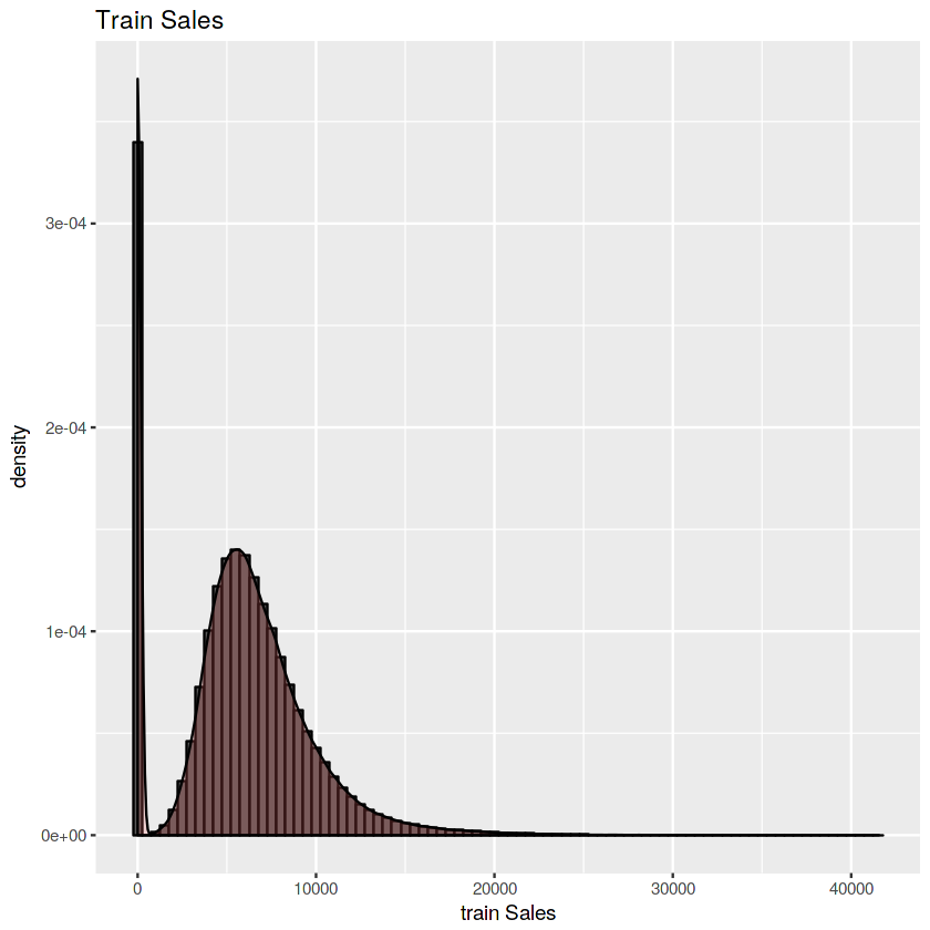
#학교휴일 여부에 따른 판매량 ???...
ggplot(train[Sales != 0], aes(x = factor(SchoolHoliday), y = Sales)) +
  geom_jitter(alpha = 0.1) +
  geom_boxplot(color = "yellow", outlier.colour = NA, fill = NA) +
    geom_hline(yintercept = 6500, size = 1, linetype = 3, color = "#FFA500")   # 오렌지색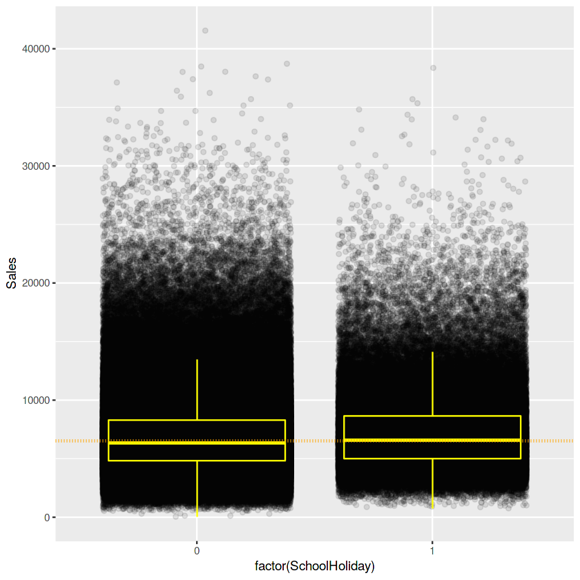
위 박스플롯으로 학교 휴일여부에 따른 Rossman 가게들의Sales를 check했고,
Sales & Customers가 0 이 아닌 train 데이터를 가지고 scatter plot을 그려보겠습니다.
ggplot(train[train$Sales != 0 & train$Customers != 0], aes(x = Customers, y = Sales)) +
  geom_point(alpha = 0.2) +
  geom_smooth() +
  geom_text_repel(aes(label = ifelse(train$Customers[train$Sales != 0 & train$Customers != 0]>6000, rownames(train), '')))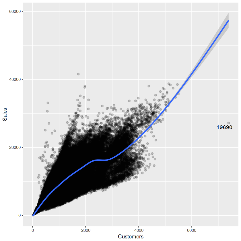
ggplot(train[train$Sales != 0 & train$Customers != 0], aes(x = log(Customers), y = log(Sales))) +
  geom_point(alpha = 0.2) +
  geom_smooth()
#당연한 얘기지만 역시 Customers가 많아야 Sales가 많다는 건 당연한건가보네요.
#마치 y=x같은 그래프와 유사한 모습을 보여주네요. 상관분석을 했는데 이렇게 이쁘게 나오면 참 기분이 좋을텐데 여튼 넘어가겟습니다.
#sales의 log를 취하는 이유는 정규분포~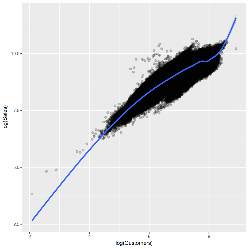
#Promo  행사여부에 따른 판매량 추이
ggplot(train[train$Sales != 0 & train$Customers != 0], aes(x = factor(Promo), y = Sales)) +
    geom_jitter(alpha = 0.1) +
    geom_boxplot(color = "yellow", outlier.colour = NA, fill = NA)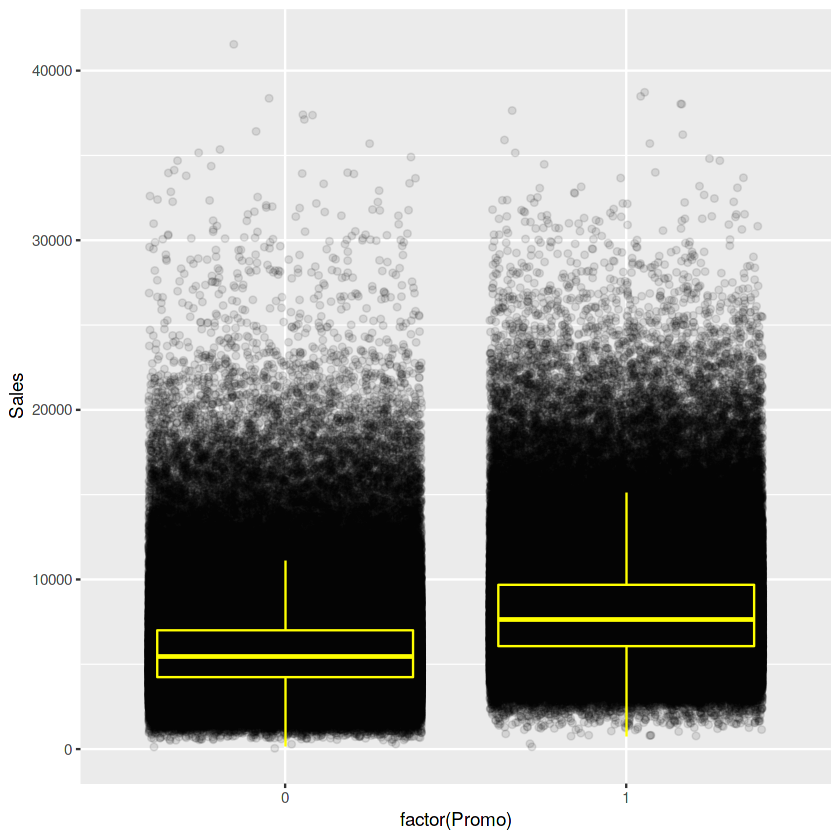
그리고 Customers과 promo를 비교함으로써 얼마나 관계가 있는지 확인.
ggplot(train[train$Sales != 0 & train$Customers != 0],
       aes(x = factor(Promo), y = Customers)) +
    geom_jitter(alpha = 0.1) +
    geom_boxplot(color = "yellow", outlier.colour = NA, fill = NA)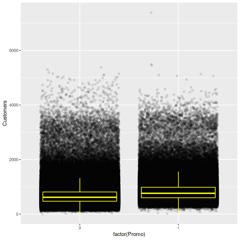
절대적이진 않지만 학교휴무여부보다 프로모션여부가 확실히 판매량 차이가 더 극명하네요
Sales와 Customers가 0인것은 제외를 함으로써 biased될 가능성이 있기 때문이라고 합니다. ????
Note: I chose to not plot that data including days with 0 sales or customers because that would have biased the boxplots. ??? 무슨말일까요 ???
판매량은 고객수와 연관이 있는데, promo여부에 따른 고객수의 차이는 거의 없습니다. 하지만, 위에 위에 plot에서는 sales가 증가하는데,
그 이유는 promo여부가 고객 한 사람이 소비하는 소비량이 증가한다는 의미입니다.
# with() : with( )는 데이터 프레임 또는 리스트 내 필드를 필드 이름만으로 접근할 수 있게 해주는 함수다.
# https://thebook.io/006723/ch04/08/01/
with(train[train$Sales != 0 & train$Promo == 0], mean(Sales / Customers))

with(train[train$Sales != 0 & train$Promo == 1], mean(Sales / Customers))


table(ifelse(train$Sales != 0, "Sales > 0", "Sales = 0"), ifelse(train$Promo, "Promo", "No promo"))
8.94112769672488
10.1789609095826
No promo Promo
Sales = 0 161666 11205
Sales > 0 467463 376875Sales = 0 일때 promo인 경우 가 있음. 위에서 조사했을때는 11196인데 9개정도 차이가 남. 왜지 하고 open에 대한 것 조사.
가게들이 문을 닫았을 때 프로모션기간인 경우가 좀 있네요 그리고 가게 문을 열었을 경우 45프로의 가게가 프로모션 진행중이구요
table(ifelse(train$Open == 1, "Opened", "Closed"), ifelse(train$Sales > 0, "Sales > 0", "Sales = 0"))

# That tends to happen on consecutive days. Some stores even had customers # (who bought nothing?) train[Open == 1 & Sales == 0]
# 다음은 웃픈 얘기인데 오픈해서 손님이 있어도 판매가 없는 가게가 54곳이나 뽑히네요.
Sales = 0 Sales > 0
Closed 172817 0
Opened 54 844338# 가슴 아프지만 우리는 이 가게들을 캐내서 판매부진 아니.. 판매불능의 상황을 따져봅시다...!! 우선 Store의 리스트를 가져와 sales가 0인것들이
# 이거는 이해 하기 힘드니 Rstudio랑 같이 보여주기!!!
zerosPerStore <- sort(tapply(train$Sales, list(train$Store), function(x) sum(x == 0)))
hist(zerosPerStore,100)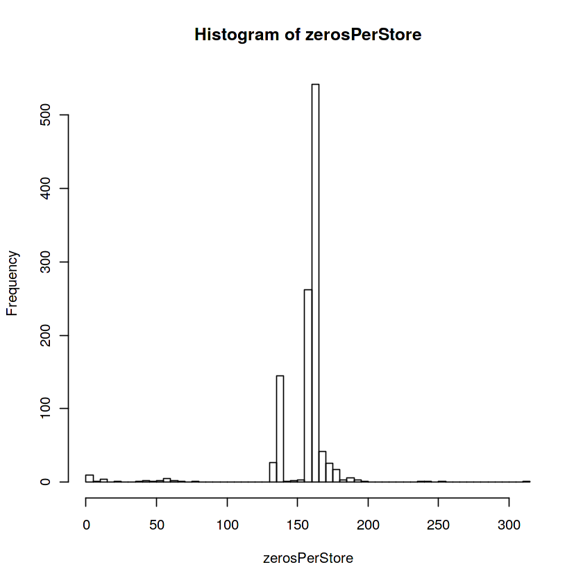
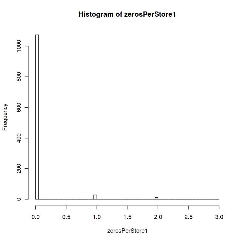
train1 <- train  %>% filter(Open == 1)
zerosPerStore1 <- sort(tapply(train1$Sales, list(train1$Store), function(x) sum(x == 0)))
which(zerosPerStore1 != 0) # 왼쪽값이 store이고 오른쪽이 sort된거인데 첨보고 헷갈림..57 1075
227 1076
232 1077
238 1078
259 1079
.
.
.
1039 1113
1100 1114
28 1115hist(zerosPerStore1,100)
가게별 판매가 0인 날로 그치는 날수가 제일 많은게 160~200일 동안 장사가 안되는 날이 있음. 하지만 여기에는 open 하지 않은 자료도 포함되어있다는게 함정(?)
여기에서는 이 구한 zerosPerStore은 sort가 되어 있죠 default가 ascending order라 판매가 0인 날이 가장 많은 가게들 10개를 가져와봅니다. 그리고 그 가게별로 plot을 찍어보네요 Sales에 대한 plot을 찍고 보니 특정 구간에 판매량이 0으로 몰린다는겁니다. 중간에 뻥 아니면 시작부분에 뻥 (?아직 이해 못함)
# Stores with the most zeros in their sales:
tail(zerosPerStore, 10) #왼쪽이 store, 오른쪽이 sale = 0 갯수
105 188
339 188
837 191
25 192
560 195
674 197
972 240
349 242
708 255
103 311tail(zerosPerStore1, 10)339 2
364 2
623 2
665 2
835 2
983 2
1017 2
1039 2
1100 2
28 3# Some stores were closed for some time, some of those were closed multiple times
plot(train[Store == 972, Sales], ylab = "Sales", xlab = "Days", main = "Store 972")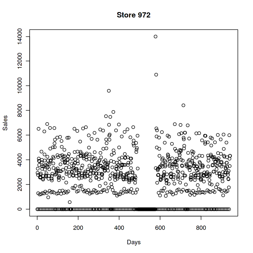
plot(train[Store == 349, Sales], ylab = "Sales", xlab = "Days", main = "Store 349")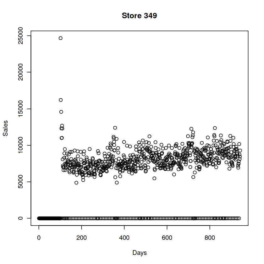
plot(train[Store == 103, Sales], ylab = "Sales", xlab = "Days", main = "Store 103")
# 여담이지만 103하고 349 되게 비슷하네요...?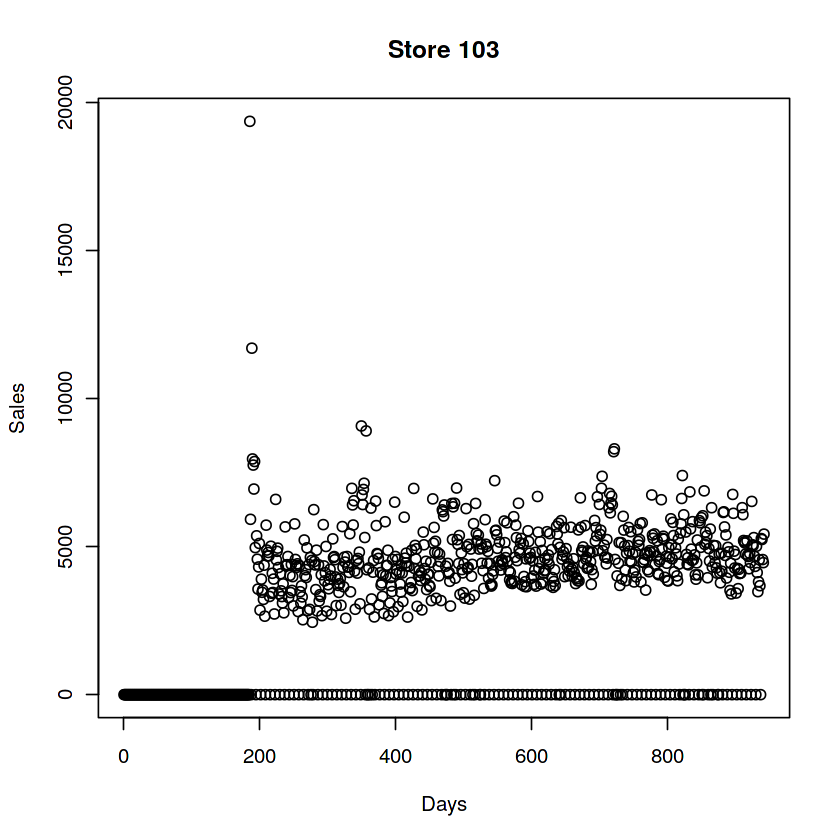
plot(train[Store == 708, Sales], ylab = "Sales", xlab = "Days", main = "Store 708")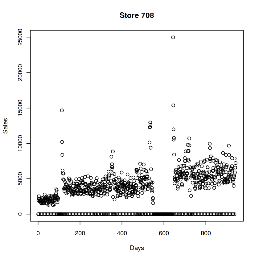
There are also stores that have no zeros in their sales. These are the exception
since they are opened also on sundays / holidays. The sales of those stores
on sundays are particularly high:
1111 0
1112 0
1113 0
1114 0
1115 0
877 22
433 71
931 80
867 85
299 86
524 86
209 87
732 88
1045 88
122 90
453 92
863 92
1099 96
310 102
512 106
530 106
578 106
1081 108
676 131
948 132
259 133
274 133
353 133
85 134
262 134
335 134
423 134
494 134
562 134
682 134
733 134
769 134
1097 134
#물론 판매량에 있어 0을 안 찍은 가게들도 있고 일요일/휴무일날 오픈해서 판매한 exceptions들도 있다고 합니다. 특히 일요일은 판매가 잘된다고 하네요..
ggplot(train[Store == 85], aes(x = Date, y = Sales, color = factor(DayOfWeek == 7), shape = factor(DayOfWeek == 7))) +
geom_point(size = 3) +
ggtitle("Sales of store 85 (True if sunday)")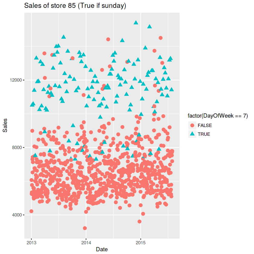
ggplot(train[Store == 262], aes(x = Date, y = Sales, color = factor(DayOfWeek == 7), shape = factor(DayOfWeek == 7))) +
    geom_point(size = 3) +
    ggtitle("Sales of store 262 (True if sunday)")

#그리고 주일별로 한번 판매량을 boxplot찍어보니!!! 일요일은 판매량의 변동성이 꽤 높네요 ㄷㄷㄷㄷ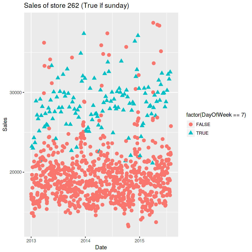
ggplot(train[Sales != 0], aes(x = factor(DayOfWeek), y = Sales)) +
    geom_jitter(alpha = 0.1) +
    geom_boxplot(color = "yellow", outlier.colour = NA, fill = NA)
# 일요일은 다들 쉬어서 그렇다 치고, 월요일은 일요일 쉬고 그 다음날이라 그런듯.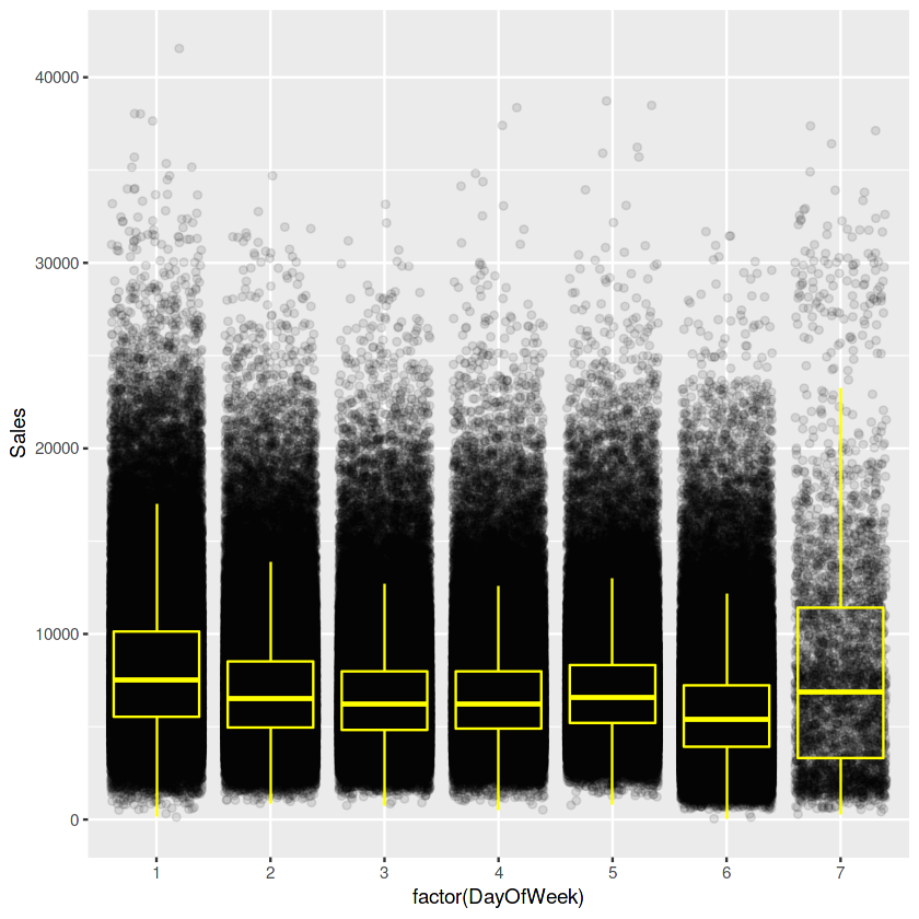
자 이제 train데이터는 그만 잠시 접어두고 주어진 데이터 셋중에 store 즉   가게 자체애 대한 정보를 받았죠. 가게 대장이라고 부를께요.

이데이터를summary()함수를 통해서 살펴보겠습니다.


summary(store)


1115개의 가게별로 StoreType / Assortment 같은 구분이 있고 경쟁업체 위치 그리고 경쟁업체 오픈 년월과 Promotion 에대한 추가 정보가 있네요. 프로모션2는 뭐지? 흠흠..

```StoreType``` - differentiates between 4 different store models: a, b, c, d<br>
```Assortment``` - describes an assortment level: a = basic, b = extra, c = extended<br>
```CompetitionDistance``` - distance in meters to the nearest competitor store<br>
```CompetitionOpenSince[Month/Year]``` - gives the approximate year and month of the time the nearest competitor was opened<br>
```Promo``` - indicates whether a store is running a promo on that day<br>
```Promo2``` - Promo2 is a continuing and consecutive promotion for some stores: 0 = store is not participating, 1 = store is participating<br>
```Promo2Since[Year/Week]``` - describes the year and calendar week when the store started participating in Promo2<br>
```PromoInterval``` - describes the consecutive intervals Promo2 is started, naming the months the promotion is started anew. E.g. "Feb,May,Aug,Nov" means each round starts in February, May, August, November of any given year for that store<br>
summary(store) Store StoreType Assortment CompetitionDistance
Min. : 1.0 Length:1115 Length:1115 Min. : 20.0
1st Qu.: 279.5 Class :character Class :character 1st Qu.: 717.5
Median : 558.0 Mode :character Mode :character Median : 2325.0
Mean : 558.0 Mean : 5404.9
3rd Qu.: 836.5 3rd Qu.: 6882.5
Max. :1115.0 Max. :75860.0
NA's :3
CompetitionOpenSinceMonth CompetitionOpenSinceYear Promo2
Min. : 1.000 Min. :1900 Min. :0.0000
1st Qu.: 4.000 1st Qu.:2006 1st Qu.:0.0000
Median : 8.000 Median :2010 Median :1.0000
Mean : 7.225 Mean :2009 Mean :0.5121
3rd Qu.:10.000 3rd Qu.:2013 3rd Qu.:1.0000
Max. :12.000 Max. :2015 Max. :1.0000
NA's :354 NA's :354
Promo2SinceWeek Promo2SinceYear PromoInterval
Min. : 1.0 Min. :2009 Length:1115
1st Qu.:13.0 1st Qu.:2011 Class :character
Median :22.0 Median :2012 Mode :character
Mean :23.6 Mean :2012
3rd Qu.:37.0 3rd Qu.:2013
Max. :50.0 Max. :2015
NA's :544 NA's :544 table(store$StoreType) a b c d
602 17 148 348table(store$Assortment) a b c
593 9 513# There is a connection between store type and type of assortment
table(data.frame(Assortment = store$Assortment, StoreType = store$StoreType)) StoreType
Assortment a b c d
a 381 7 77 128
b 0 9 0 0
c 221 1 71 220hist(store$CompetitionDistance, 100)
#경쟁업체거리는 있다면 뭐 가까운데 제일 많이 있다라는거죠 거리가 멀수록 경쟁업체가 있어도 없다고 체크합니다. (관리상...)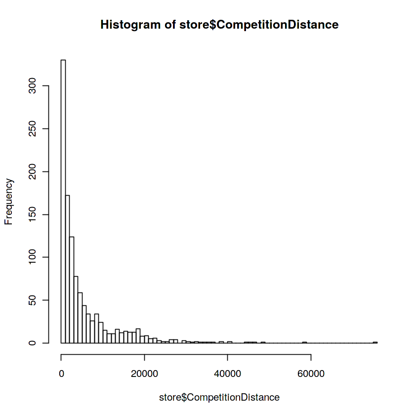
#뭐 이건 년월을 "-"로 묶어서 CompetitoinOpenSince라는 값에 담았습니다. 그리고 2015년 10월 기준으로 오픈한 년수를 구해서 historgram으로 찍어봤을때 보통 20년 이내의 역사를 가지고 있는 가게가 대부분이네요.

# Convert the CompetitionOpenSince... variables to one Date variable

store$CompetitionOpenSince <- as.yearmon(paste(store$CompetitionOpenSinceYear, store$CompetitionOpenSinceMonth, sep = "-"))
# One competitor opened 1900 hist(as.yearmon("2015-10") - store$CompetitionOpenSince, 100, main = "Years since opening of nearest competition")
Promo2 : Promo2 is a continuing and consecutive promotion for some stores: 0 = store is not participating, 1 = store is participating
Promo2Since[Year/Week] : describes the year and calendar week when the store started participating in Promo2
# Assume that the promo starts on the first day of the week
store$Promo2Since <- as.POSIXct(paste(store$Promo2SinceYear, store$Promo2SinceWeek, 1, sep = "-"), format = "%Y-%U-%u")
hist(as.numeric(as.POSIXct("2015-10-01", format = "%Y-%m-%d") - store$Promo2Since),
     100, main = "Days since start of promo2")
# 이런거 보면 오픈기간에 따른 sales를 분석해보는것도 의미있을것 같아욤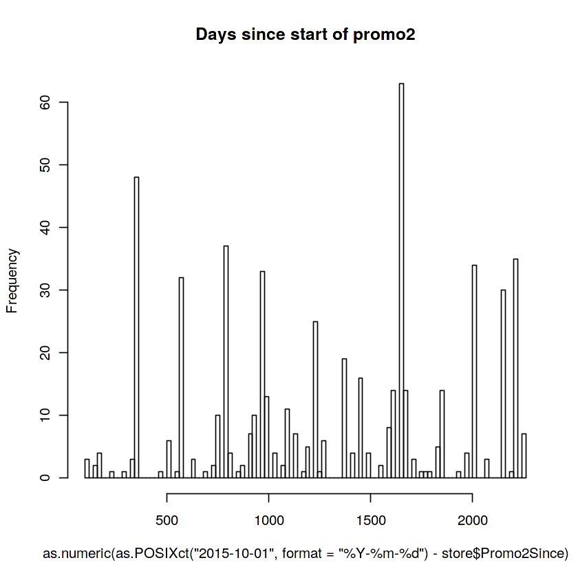
#1. 프로모션 주기구요.

table(store$PromoInterval)

#1월,Jan
#2월,Feb
#3월,Mar
#4월,Apr
#5월,May
#6월,June
#7월,July
#8월,Aug
#9월,Sept
#10월,Oct
#11월,Nov
#12월Dec
Feb,May,Aug,Nov Jan,Apr,Jul,Oct Mar,Jun,Sept,Dec
544 130 335 106# Merge store and train
train_store <- merge(train, store, by = "Store")
ggplot(train_store[Sales != 0], aes(x = factor(PromoInterval), y = Sales)) +
geom_jitter(alpha = 0.1) +
geom_boxplot(color = "yellow", outlier.colour = NA, fill = NA)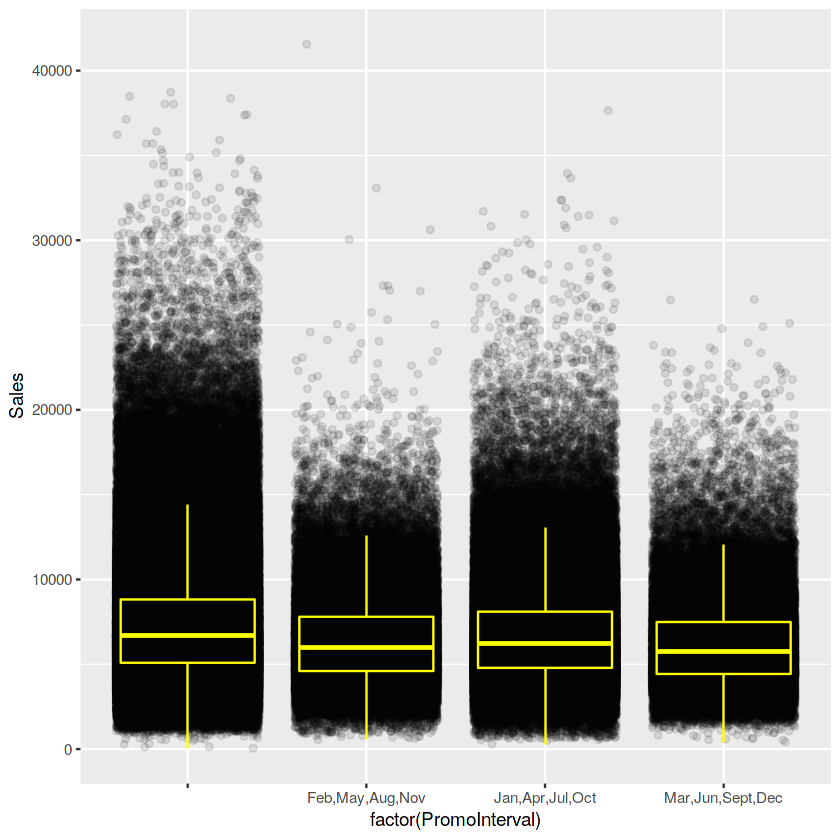
store type과 assortment types을 시각분석을 통해 확인.
그래프가 마치 지렁이같이 그려지는건 geom_smooth 때문이고 여튼 factor를 storeType과 assortment type을 넣고 덜리기.
store type : differentiates between 4 different store models: a, b, c, d
assortment types: describes an assortment level: a = basic, b = extra, c = extended
ggplot(train_store[Sales != 0],aes(x = as.Date(Date), y = Sales, color = factor(StoreType))) + geom_smooth(size = 2)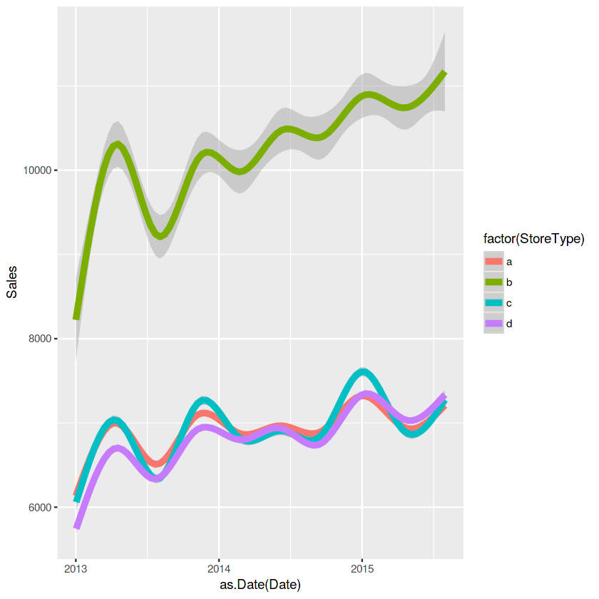
ggplot(train_store[Customers != 0], aes(x = as.Date(Date), y = Customers, color = factor(StoreType))) + geom_smooth(size = 2)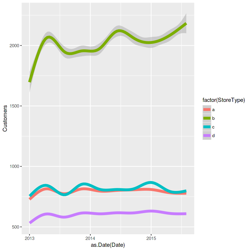
#고객 수랑 sales 비율 비교하는것도 재밌을듯
ggplot(train_store[Sales != 0], aes(x = as.Date(Date), y = Sales, color = factor(Assortment))) + geom_smooth(size = 2)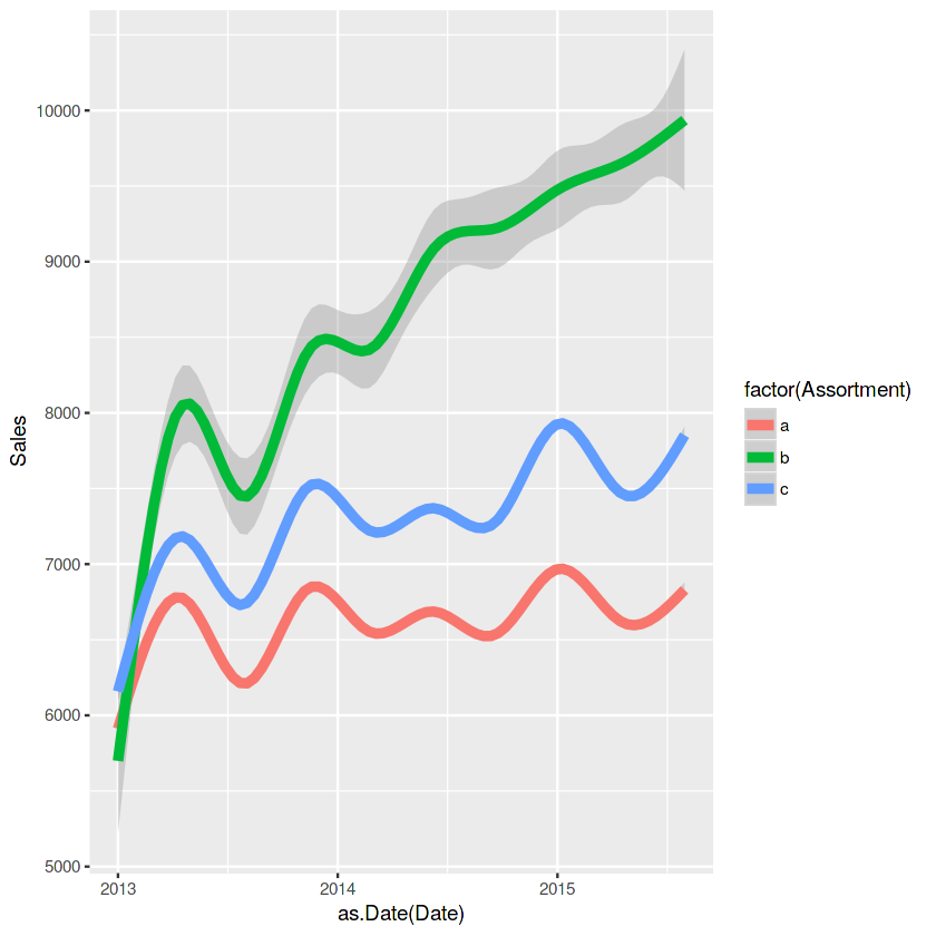
ggplot(train_store[Sales != 0], aes(x = as.Date(Date), y = Customers, color = factor(Assortment))) + geom_smooth(size = 2)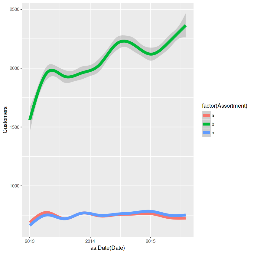
storetype과 assortment type을 보면 b가 우세하네요. 고객수면이나 판매량측면에서 말이죠!!
경쟁업체와의 거리는 좀 보면 직관적이지 못합니다. 경쟁업체와의 거리가 가까운 가게의 경우는 일반적으로 도심지역으로 customers 또한 많다. 그래서 good bad를 가리기엔 cancel out 즉 ,상쇄가 된다.
salesByDist <- aggregate(train_store[Sales != 0 & !is.na(CompetitionDistance)]$Sales,
               by = list(train_store[Sales != 0 & !is.na(CompetitionDistance)]$CompetitionDistance), mean)
colnames(salesByDist) <- c("CompetitionDistance", "MeanSales")
ggplot(salesByDist, aes(x = log(CompetitionDistance), y = log(MeanSales))) +
    geom_point() + geom_smooth()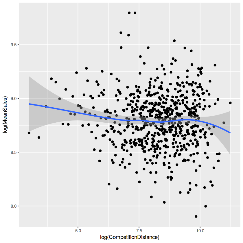
# CompetitionOpenSinceYear값이 없을 경우때문인지 걍 CompetitionOpenSinceYear의 값 존재여부를 가지고 체크한거같습니다. 보시죠.

ggplot(train_store[Sales != 0],
       aes(x = factor(!is.na(CompetitionOpenSinceYear)), y = Sales)) +
    geom_jitter(alpha = 0.1) +
    geom_boxplot(color = "yellow", outlier.colour = NA, fill = NA) +
    ggtitle("Any competition?")
#별차이가 없어보이는데 우선 뭐.. Sales가 있는경우가 더 높네요. 방금 말한 그런 이유의 연장선인거같습니다
# http://verystrongjoe.tistory.com/entry/Kagglers-Day-8?category=509908 한글자료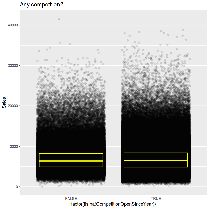
So what happens if a competitor opens? In order to assess this effect we fetch
data from all stores that first have NA as CompetitorDistance and later some
value. Only the month, not the date, of the opening of the competitor is known
so we need a rather large window to see the effect (100 days). 147 stores
had a competitor move into their area during the available time span. The
competition leaves a 'dent' in the sales which looks a little different
depending on the chosen timespan so I wouldn't like to argue about statistical
significance based on this plot alone. It's informative to look at anyway:
경쟁업체가 오픈하면 어떤일이 벌어질까요? 이 효과를 평가하기 위해 우리는 가게중 처음 CompetitorDistance 의 값이 NA로 되어 있다가 후에 의미있는값으로 채워지는 것을 가져옵니다.
특정 날짜가 아닌 경쟁업체의 개업 달만 알려져있다고 합니다.
147개의 가게가 이용가능한 기간동안 그들의 영역에 옮겨왔다고 합니다. 이 경쟁은 기간을 어떻게 잡느냐에 따라 달라지는 판매량에서 움픅 들어간 모습을 보여준답니다.
# Sales before and after competition opens
train_store$DateYearmon <- as.yearmon(train_store$Date) # 소스가 길어 주석을 달자면 월로 truncate
train_store <- train_store[order(Date)] #  R을 보면서 항상 이런게 대박인것 같습니다. vectorize연산이 이리 쉽게 되죠. Date순으로 order줍니다.
timespan <- 100 # Days to collect before and after Opening of competition
beforeAndAfterComp <- function(s) {
x <- train_store[Store == s]
daysWithComp <- x$CompetitionOpenSince >= x$DateYearmon
if (any(!daysWithComp)) {
compOpening <- head(which(!daysWithComp), 1) - 1
if (compOpening > timespan & compOpening < (nrow(x) - timespan)) {
x <- x[(compOpening - timespan):(compOpening + timespan), ]
x$Day <- 1:nrow(x)
return(x)
}
}
}temp <- lapply(unique(train_store[!is.na(CompetitionOpenSince)]$Store), beforeAndAfterComp)
temp <- do.call(rbind, temp)
# 147 stores first had no competition but at least 100 days before the end
# of the data set
length(unique(temp$Store))147
ggplot(temp[Sales != 0], aes(x = Day, y = Sales)) +
    geom_smooth() +
    ggtitle(paste("Competition opening around day", timespan))

#확실히 전후로 매출에 변화가 급감하였다가  다시 회복하는 기조를 보이네요..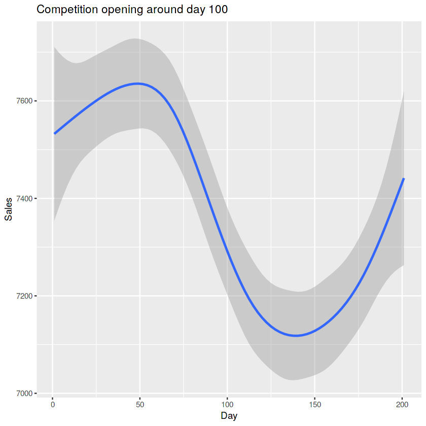
The seasonplot is adapted from spsrini
(edit: Replace sum and show sales in relation to mean daily sales of a store which
better accounts for missing data / closed stores):
#다른 plot을 가져옵니다. Seaonal plot(spsrini)이라고 합 대신에 missing value나 closed store 대신하여 더 값을 잘표현할수 있는 평균값으로 보여주는 plot이라고 합니다.

#판매량 평균값으로 계절 추이를 볼수 있는거 같습니다.

temp <- train
temp$year <- format(temp$Date, "%Y")
temp$month <- format(temp$Date, "%m")
temp[, StoreMean := mean(Sales), by = Store]
temp <- temp[, .(MonthlySalesMean = mean(Sales / (StoreMean)) * 100),
             by = .(year, month)]
temp <- as.data.frame(temp)
SalesTS <- ts(temp$MonthlySalesMean, start=2013, frequency=12)
col = rainbow(3)
seasonplot(SalesTS, col=col, year.labels.left = TRUE, pch=19, las=1)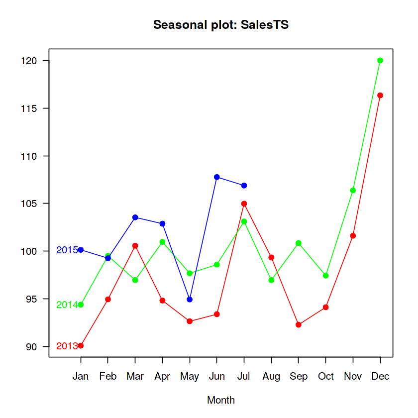
7.추가사항
- 1. dplyr의 lag를 이용해서 전날 customer 여부 or 일주일마다 cum으로 고객수 check. 왜냐하면 나를 생각했을때 일주일에 한번 정도 마트를 가니깐 한번 간사람은 일주일 이내에는 다시 잘 안갈거라는 생각으로...? 근데 약국을 주기적으로 가나?? -- 데이터가 많으면 정규분포 따를거 같기도 함.
- 2. 전날 일요일이 열었는지 휴일이 열었는지도 의미가 있을듯. 아니면 다음날이 휴일이거나 하는것도... ( 다음날 일요일인것은 왜인지는 모르겠지만 값이 떨어짐. 아마 쉬어서 그런가...? / 반대로 월요일 같은 경우는 전날 쉬었기에 값이 오르고, 마찬가지로 일요일ㄷ ㅗ값이 오름. )
- 3. 경쟁업체의 customers이 증가하면 우리 가게의 customers수는 감소하지 않을까???
- 4. 고객당 판매비율
- 5. store 시간에 대한 판매량 ?
- 6. store 요일 마다 평균, 분산
- 7. 오픈기간에 따른 sales를 분석해보는것도 의미있을것 같아욤
- 8. group by를 통해 store종류랑 요일 등등을 묶는것도 의미있어보임!~
time-series-analysis-and-forecasts-with-prophet
time-series-analysis
다음주차로는 다른사람들의 EDA자료를 정리해보도록 하겠습니다.
'TEAM EDA > EDA 1기 ( 2018.03.01 ~ 2018.09.16 )' 카테고리의 다른 글
| kaggle - Rossmann Store sales Prediction (3) (0) | 2019.09.10 |
|---|---|
| kaggle - Rossmann Store sales Prediction (2) (1) | 2019.09.10 |
| Decision Tree (의사결정나무) (0) | 2019.09.10 |
| linear regression (선형회귀분석) with R (0) | 2019.09.10 |
| 결측치 처리 (Missing Value) (3) | 2018.11.12 |


