
| 일 | 월 | 화 | 수 | 목 | 금 | 토 |
|---|---|---|---|---|---|---|
| 1 | 2 | 3 | ||||
| 4 | 5 | 6 | 7 | 8 | 9 | 10 |
| 11 | 12 | 13 | 14 | 15 | 16 | 17 |
| 18 | 19 | 20 | 21 | 22 | 23 | 24 |
| 25 | 26 | 27 | 28 | 29 | 30 | 31 |
- DilatedNet
- 알고리즘
- 큐
- 코딩테스트
- 한빛미디어
- Python
- 엘리스
- 파이썬
- Object Detection
- hackerrank
- 3줄 논문
- MySQL
- 프로그래머스
- pytorch
- Segmentation
- Recsys-KR
- Image Segmentation
- Semantic Segmentation
- DFS
- 추천시스템
- 나는리뷰어다
- eda
- 스택
- 입문
- 나는 리뷰어다
- TEAM-EDA
- Machine Learning Advanced
- 협업필터링
- TEAM EDA
- 튜토리얼
- Today
- Total
TEAM EDA
[kaggle] KUC Hackathon Winter 2018 : What can you do with the Drug Review dataset? 본문
[kaggle] KUC Hackathon Winter 2018 : What can you do with the Drug Review dataset?
김현우 2020. 3. 23. 08:54지난 House price Advanced Regression에 이어 이번 EDA 2기 두번째 프로젝트로 진행했던 KUC Hackathon Winter 2018 : What can you do with the Drug Review dataset?(https://www.kaggle.com/jessicali9530/kuc-hackathon-winter-2018)에 대한 분석 보고서입니다.
(+추가) 이번 해커톤 우승팀중 하나인 저희팀의 인터뷰입니다.(http://blog.kaggle.com/2019/01/14/kuc-teameda/)

이번 대회는 캐글을 하는 대학생팀들을 위한 해커톤으로 따로 문제가 있는 것이 아니라 팀별로 주제를 선정해서 한달 동안 각자의 분석을 진행하는 대회였습니다. 개인적으로 자연어처리라는 분야에 대해 처음 하는것이라 여러분들이 보기에 이상한 부분이 있을 수 있습니다. 그러한 부분은 댓글로 피드백 남겨주시면 공부해보고 수정해보도록 하겠습니다.
저희 팀은 리뷰 및 감성분석을 통한 환자의 상태에 맞는 약을 추천하는 주제를 잡고 진행했습니다. 진행 과정은 데이터 탐색 - 데이터 전처리 - 모델 - 결론 - 한계 순으로 진행됩니다. 데이터 탐색 부분에서는 시각화 기법과 통계적인 기법으로 데이터의 형태에 대해 살펴봅니다. 이러한 과정을 통해서 주제를 정할 수 있었고 주제에 맞게끔 데이터를 전처리하고 다양한 변수를 만들어서 모델을 만듭니다. 이때, 단어사전을 이용한 감성분석, 딥러닝을 적용한 n-gram 등을 사용하였고 자연어처리의 한계를 보완하기 위해 Lightgbm이라는 머신러닝 모델을 도입하고 추가적으로 추천수를 통하여 신뢰성을 보장하였습니다. 마지막으로 프로젝트에 대한 결론과 분석을 진행하면서 아쉬웠던 점이나 부족했던 점을 한계점을 소개합니다.
1. 데이터 탐색 (Exploration Data Analysis)
1.1. 데이터 이해
먼저 Train데이터와 Test 데이터를 불러오도록 하겠습니다. 두 데이터의 크기는 아래와 같고 데이터의 출처를 살펴 본 결과
https://archive.ics.uci.edu/ml/datasets/Drug+Review+Dataset+%28Drugs.com%29에 올라와 있는 데이터였고 online pharmaceutical review sites에 있는 리뷰들을 크롤링하여 만든 데이터였습니다.
Train shape : (161297, 7)
Test shape : (53766, 7)
head() 명령어를 통해 데이터를 살펴 본 결과입니다. 개인을 식별해주는 uniqueID를 제외하고 총 6개의 변수가 있고 review가 핵심적인 변수임을 확인할 수 있습니다.

추가적으로 변수 설명은 아래와 같습니다.
- drugName (categorical): name of drug
- condition (categorical): name of condition
- review (text): patient review
- rating (numerical): 10 star patient rating
- date (date): date of review entry
- usefulCount (numerical): number of users who found review useful
데이터의 구조는 uniqueID를 가진 환자가 자신의 condition에 맞는 drug를 구매하고, date에 자신이 산 drug에 대해 review와 rating을 적습니다. 그 다음에 이 리뷰를 본 사람들이 리뷰가 도움이 되면 usefulCount를 클릭해서 +1씩 되는 구조입니다.
1.2. 변수 이해
먼저 uniqueID부터 차례대로 변수 탐색을 시작하도록 하겠습니다. 동일한 고객이 여러번의 리뷰를 작성했는지 확인하기 위해 uniqueID의 unique한 갯수와 트레인 데이터의 길이를 비교해 본 결과 동일한 고객은 데이터에 존재하지 않았습니다.

drugName은 condition과 밀접한 관련이 있기에 같이 분석을 진행했습니다. 두 변수의 unique values는 각각 3671, 917로 하나의 상태마다 4개정도의 약이 존재합니다. 이를 보다 자세히 보기 위해 시각화를 진행해보도록 하겠습니다.

위의 그림을 보면 알겠지만, 상위 8개의 약은 condition 당 약의 갯수가 약 100개 정도가 넘습니다. 그런데 주목할 만한 점은 3</span> users found this comment helpful 이라는 문장이 condition에 등장하는데 이는 크롤링 과정에서 생긴 오류 같습니다. 보다 자세히 확인하기 위해서 아래와 같이 살펴봤습니다.

이는 usefulCount </span> users found this comment helpful. 의 구조로 3만 있는게 아니라 위에 그림처럼 4도 있을것이고 다른 숫자들도 있을것으로 예상되어집니다. 이러한 데이터는 추후 전처리 과정에서 제거하도록 하겠습니다.
다음은 drugs per condition의 하위 20개의 condition 입니다. 보면 알겠지만, 모두 갯수가 1개로 동일합니다. 추천시스템을 생각했을 때, 과연 한개의 상품만 있는데 이를 추천하는게 옳은지 고민해보면 조금 갸우뚱합니다. 그래서 condition 당 최소 2개 이상의 약이 존재하는 condition만을 뽑아서 분석을 진행하도록 하겠습니다.

다음으로는 review에 대해 보도록 하겠습니다. 먼저 눈에 띄는 부분은 \r \n 과 같은 html문자열이 보이고, MUCH와 같은 대문자로 강조표시와 (very unusual for him), (a good thing) 과 같은 감성을 표현하는 부분이 괄호안에 들어가 있습니다.

추가적으로 다음 리뷰를 살펴봤을 때, didn't가 didn't로 표기 되어 있다든지, ...와 같은 특수문자들도 확인할 수 있습니다.

이러한 부분도 전처리 할 떄 추가적으로 제거하도록 하겠습니다.
다음으로는 WordCloud 부분 입니다. 어떠한 값들이 많이 나온지 가볍게 확인해볼 수 있습니다.

다음으로는 rating 1~5를 부정, 6~10을 긍정으로 Category화 하고 두개의 감성별 n-gram을 살펴보도록 하겠습니다.

1-gram을 사용했을떄, 상위5개의 단어를 보면 왼쪽과 오른쪽이 순서는 다르지만 내용은 똑같은 것을 확인할 수 있습니다. 이는 하나의 말뭉치로 텍스트 분석을 했을 때, 감성을 잘 분류하지 못한다는 의미로 말뭉치를 좀 더 확장하도록 하겠습니다

Bigram 또한 마찬가지로 상위 5개의 내용이 비슷하고 읽어봤을 때, 긍정과 부정을 분류하기 힘든 뭉치입니다. 추가적으로 side effects 와 side effects.이 다르게 해석되는걸로 봐서 전처리 부분이 필요합니다. 그리고 side effects, weight gain, highly recommend 처럼 이전 1-gram보다는 감성을 분류할 만한 뭉치들이 나오는것을 볼 수 있습니다.

Tri-gram 부터는 말뭉치와 긍-부정사이가 보이는 것을 알 수 있습니다. bad side effects라든지 birth control pills, negative side effects 모두 금-부정을 분류하는 뭉치입니다. 하지만 긍정을 나타내는 부분과 부정을 나타내는 부분에 모두 있어서 앞의 not이라든지 어떠한 조사에 의해 내용이 반전 되는 부분이 빠져있다는 것을 생각할 수 있습니다.

확실히 4-gram이 다른 gram보다 감성의 분류가 잘 된 것을 볼 수 있습니다. 최종적으로는 4-gram을 이용하여 딥러닝 모델을 만들어보도록 하겠습니다. 다음으로는 rating과 날짜들 사이의 관계에 대해 살펴보도록 하겠습니다.
먼저 rating의 갯수부터 세보도록 하겠습니다.

대부분의 사람들이 10,9,1,8 이라는 4개의 값을 많이 고르고 그 중 10은 다른 값들의 2배이상입니다. 이걸로 봤을 때, 부정보다는 선호의 비율이 높고 사람들의 반응이 극단적이라는것을 확인할 수 있습니다.
다음으로 날짜에 따라 리뷰의 갯수와 rating의 비율을 살펴보도록 하겠습니다.


재미있는 점은 연도별로는 평균 레이팅이 다른게 눈에 보이지만, 월별로는 평균 레이팅이 비슷한것을 확인 할 수 있습니다.

월급일같이 요일이 rating에 영향을 미치는지 살펴봤으나 미세하게 차이는 있지만 큰 차이를 보이지는 않습니다.
다음으로는 리뷰의 유의미함을 판단하는 척도인 Usefulcount입니다.


usefulCount의 분포를 살펴봤을때, 최솟값이 0 부터 최댓값은 1291까지 최소와 최대의 차이가 큰 것을 볼 수 있습니다. 추가적으로 편차 또한 36으로 생각보다 큰 값입니다. 이러한 이유는 사람들이 많이 찾는 drug일 수록 내용이 좋든 나쁘든 보는 사람이 많으니깐 usefulcount가 높을 수 밖에 없습니다. 그래서 추후에 모델을 만들어 줄때는 이러한 부분을 사람들이 찾는 비율에 맞게 끔 정규화시켜주도록 하겠습니다.
1.3 결측치 (Missing values)

Missing value (%): 0.5579760349292998 으로 전체의 1%도 되지 않으니 제거하도록 하겠습니다.
2. 데이터 전처리 (Data Preprocessing)
2.1 결측치(Missing value) 제거
df_train = df_train.dropna(axis=0)
df_test = df_test.dropna(axis=0)
2.2 상태(Condition) 전처리
먼저 3</span> users found this comment helpful. 와 같은 형식의 문장들을 제거하도록 하겠습니다.
all_list = set(df_all.index)
span_list = []
for i,j in enumerate(df_all['condition']):
    if '</span>' in j:
        span_list.append(i)
new_idx = all_list.difference(set(span_list))df_all = df_all.iloc[list(new_idx)].reset_index()
del df_all['index']
다음으로 condition 당 하나의 약이 존재하는 condition은 제거하도록 하겠습니다.
df_condition_1 = df_condition[df_condition['drugName']==1].reset_index()all_list = set(df_all.index)condition_list = []
for i,j in enumerate(df_all['condition']):
for c in list(df_condition_1['condition']):
if j == c:
condition_list.append(i)
new_idx = all_list.difference(set(condition_list))
df_all = df_all.iloc[list(new_idx)].reset_index()
del df_all['index']
2.3 리뷰(review) 전처리
리뷰를 전처리하는 과정은 html 문자 제거 - 특수문자 제거 - 소문자 처리 - 불용어 처리 - 어간 추출의 5단계 입니다.
먼저 불용어를 처리하기 전에 nltk에서 제공하는 불용어에 포함된 단어부터 살펴봤습니다.

내용을 보면 대부분은 이해가 가지만 needn't, 't 같이 not을 포함하고 있는 단어들이 많습니다. 이러한 단어들은 감성분석을 할 떄 핵심적인 부분이므로 불용어에서 제거하도록 하겠습니다.
not_stop = ["aren't","couldn't","didn't","doesn't","don't","hadn't","hasn't","haven't","isn't","mightn't","mustn't","needn't","no","nor","not","shan't","shouldn't","wasn't","weren't","wouldn't"]
for i in not_stop:
    stops.remove(i)
stemmer = SnowballStemmer('english')

def review_to_words(raw_review):
    # 1. HTML 제거
    review_text = BeautifulSoup(raw_review, 'html.parser').get_text()
    # 2. 영문자가 아닌 문자는 공백으로 변환
    letters_only = re.sub('[^a-zA-Z]', ' ', review_text)
    # 3. 소문자 변환
    words = letters_only.lower().split()
    # 4. 파이썬에서는 리스트보다 세트로 찾는게 훨씬 빠르다.
    # 5. Stopwords 불용어 제거
    meaningful_words = [w for w in words if not w in stops]
    # 6. 어간추출
    stemming_words = [stemmer.stem(w) for w in meaningful_words]
    # 7. 공백으로 구분된 문자열로 결합하여 결과를 반환
    return( ' '.join(stemming_words))
    #return( ' '.join(words))
%time df_all['review_clean'] = df_all['review'].apply(review_to_words)
3. 모델 (Model)
3.1 N-gram을 활용한 딥러닝
# Make a rating
df_all['sentiment'] = df_all["rating"].apply(lambda x: 1 if x > 5 else 0)

df_train, df_test = train_test_split(df_all, test_size=0.33, random_state=42)

# https://github.com/corazzon/KaggleStruggle/blob/master/word2vec-nlp-tutorial/tutorial-part-1.ipynb
from sklearn.feature_extraction.text import CountVectorizer
from sklearn.pipeline import Pipeline

vectorizer = CountVectorizer(analyzer = 'word',
                             tokenizer = None,
                             preprocessor = None,
                             stop_words = None,
                             min_df = 2, # 토큰이 나타날 최소 문서 개수
                             ngram_range=(4, 4),
                             max_features = 20000
                            )
vectorizer
#https://stackoverflow.com/questions/28160335/plot-a-document-tfidf-2d-graph
pipeline = Pipeline([
    ('vect', vectorizer),
])


%time train_data_features = pipeline.fit_transform(df_train['review_clean'])
%time test_data_features = pipeline.fit_transform(df_test['review_clean'])
from tensorflow.python.keras.models import Sequential
from tensorflow.python.keras.layers import Dense, Bidirectional, LSTM, BatchNormalization, Dropout
from tensorflow.python.keras.preprocessing.sequence import pad_sequences
#Source code in keras 김태영'blog
# 0. Package
import numpy as np
import keras
from keras.models import Sequential
from keras.layers import Dense
import random
# 1. Dataset
y_train = df_train['sentiment']
y_test = df_test['sentiment']
solution = y_test.copy()
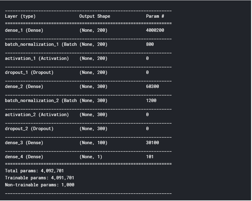
# 2. Model Structure
model = keras.models.Sequential()
model.add(keras.layers.Dense(200, input_shape=(20000,)))
model.add(keras.layers.BatchNormalization())
model.add(keras.layers.Activation('relu'))
model.add(keras.layers.Dropout(0.5))
model.add(keras.layers.Dense(300))
model.add(keras.layers.BatchNormalization())
model.add(keras.layers.Activation('relu'))
model.add(keras.layers.Dropout(0.5))
model.add(keras.layers.Dense(100, activation='relu'))
model.add(keras.layers.Dense(1, activation='sigmoid'))
# 3. Model compile
model.compile(optimizer='adam', loss='binary_crossentropy', metrics=['accuracy'])model.summary()
# 4. Train model
hist = model.fit(train_data_features, y_train, epochs=10, batch_size=64)

# 5. Traing process
%matplotlib inline
import matplotlib.pyplot as plt

fig, loss_ax = plt.subplots()

acc_ax = loss_ax.twinx()

loss_ax.set_ylim([0.0, 1.0])
acc_ax.set_ylim([0.0, 1.0])

loss_ax.plot(hist.history['loss'], 'y', label='train loss')
acc_ax.plot(hist.history['acc'], 'b', label='train acc')

loss_ax.set_xlabel('epoch')
loss_ax.set_ylabel('loss')
acc_ax.set_ylabel('accuray')

loss_ax.legend(loc='upper left')
acc_ax.legend(loc='lower left')

plt.show()

# 6. Evaluation
loss_and_metrics = model.evaluate(test_data_features, y_test, batch_size=32)
print('loss_and_metrics : ' + str(loss_and_metrics))

sub_preds_deep = model.predict(test_data_features,batch_size=32)
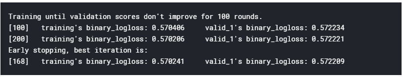
3.2 LightGBM
정확성을 높이기 위해 머신 러닝을 사용합니다. 우선, 이것은 유용한 카운트만을 사용하는 감정 분석 모델입니다.
solution = df_test['sentiment']
confusion_matrix(y_pred=sub_preds, y_true=solution)
정확도를 높이기 위해 파생변수들을 추가하겠습니다.
len_train = df_train.shape[0]
df_all = pd.concat([df_train,df_test])
del df_train, df_test;
gc.collect()
df_all['date'] = pd.to_datetime(df_all['date'])
df_all['day'] = df_all['date'].dt.day
df_all['year'] = df_all['date'].dt.year
df_all['month'] = df_all['date'].dt.monthfrom textblob import TextBlob
from tqdm import tqdm
reviews = df_all['review_clean']
Predict_Sentiment = []
for review in tqdm(reviews):
blob = TextBlob(review)
Predict_Sentiment += [blob.sentiment.polarity]
df_all["Predict_Sentiment"] = Predict_Sentiment
df_all.head()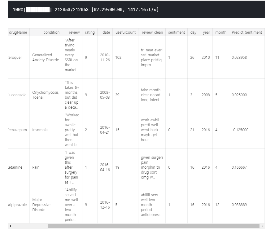
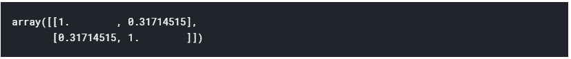
np.corrcoef(df_all["Predict_Sentiment"], df_all["rating"])

np.corrcoef(df_all["Predict_Sentiment"], df_all["sentiment"])

reviews = df_all['review']

Predict_Sentiment = []
for review in tqdm(reviews):
    blob = TextBlob(review)
    Predict_Sentiment += [blob.sentiment.polarity]
df_all["Predict_Sentiment2"] = Predict_Sentiment
np.corrcoef(df_all["Predict_Sentiment2"], df_all["rating"])

np.corrcoef(df_all["Predict_Sentiment2"], df_all["sentiment"])
#문장길이 (줄바꿈표시가 몇번나왔는지 셈)
df_all['count_sent']=df_all["review"].apply(lambda x: len(re.findall("\n",str(x)))+1)

#Word count in each comment:(단어갯수)
df_all['count_word']=df_all["review_clean"].apply(lambda x: len(str(x).split()))

#Unique word count(unique한 단어 갯수)
df_all['count_unique_word']=df_all["review_clean"].apply(lambda x: len(set(str(x).split())))

#Letter count(리뷰길이)
df_all['count_letters']=df_all["review_clean"].apply(lambda x: len(str(x)))

#punctuation count(특수문자)
df_all["count_punctuations"] = df_all["review"].apply(lambda x: len([c for c in str(x) if c in string.punctuation]))

#upper case words count(전부다 대문자인 단어 갯수)
df_all["count_words_upper"] = df_all["review"].apply(lambda x: len([w for w in str(x).split() if w.isupper()]))

#title case words count(첫글자가 대문자인 단어 갯수)
df_all["count_words_title"] = df_all["review"].apply(lambda x: len([w for w in str(x).split() if w.istitle()]))

#Number of stopwords(불용어 갯수)
df_all["count_stopwords"] = df_all["review"].apply(lambda x: len([w for w in str(x).lower().split() if w in stops]))

#Average length of the words(평균단어길이)
df_all["mean_word_len"] = df_all["review_clean"].apply(lambda x: np.mean([len(w) for w in str(x).split()]))
계절 변수를 추가하겠습니다.
df_all['season'] = df_all["month"].apply(lambda x: 1 if ((x>2) & (x<6)) else(2 if (x>5) & (x<9) else (3 if (x>8) & (x<12) else 4)))모델링

confusion_matrix(y_pred=sub_preds, y_true=solution)

cols = feature_importance_df[["feature", "importance"]].groupby("feature").mean().sort_values(
    by="importance", ascending=False)[:50].index

best_features = feature_importance_df.loc[feature_importance_df.feature.isin(cols)]

plt.figure(figsize=(14,10))
sns.barplot(x="importance", y="feature", data=best_features.sort_values(by="importance", ascending=False))
plt.title('LightGBM Features (avg over folds)')
plt.tight_layout()
plt.savefig('lgbm_importances.png')
3.3 사전을 통한 감성분석
예측에 사용 된 패키지는 영화 리뷰 데이터로 구성되므로 이 프로젝트에 적합하지 않습니다. 이를 보완하기 위해 하버드 감성 사전을 사용하여 추가적인 감성 분석을 수행했습니다.
# import dictionary data
word_table = pd.read_csv("../input/dictionary/inquirerbasic.csv")
word_table.head()

##1. make list of sentiment
#Positiv word list
temp_Positiv = []
Positiv_word_list = []
for i in range(0,len(word_table.Positiv)):
    if word_table.iloc[i,2] == "Positiv":
        temp = word_table.iloc[i,0].lower()
        temp1 = re.sub('\d+', '', temp)
        temp2 = re.sub('#', '', temp1)
        temp_Positiv.append(temp2)

Positiv_word_list = list(set(temp_Positiv))
len(temp_Positiv)
len(Positiv_word_list)  #del temp_Positiv

#Negativ word list
temp_Negativ = []
Negativ_word_list = []
for i in range(0,len(word_table.Negativ)):
    if word_table.iloc[i,3] == "Negativ":
        temp = word_table.iloc[i,0].lower()
        temp1 = re.sub('\d+', '', temp)
        temp2 = re.sub('#', '', temp1)
        temp_Negativ.append(temp2)

Negativ_word_list = list(set(temp_Negativ))
len(temp_Negativ)
len(Negativ_word_list)  #del temp_Negativ
우리는 review_clean에서 사전에 포함 된 단어의 수를 세었습니다.
##2. counting the word 98590
import numpy as np
from sklearn.feature_extraction.text import CountVectorizer

vectorizer = CountVectorizer(vocabulary = Positiv_word_list)
content = df_test['review_clean']
X = vectorizer.fit_transform(content)
f = X.toarray()
f = pd.DataFrame(f)
f.columns=Positiv_word_list
df_test["num_Positiv_word"] = f.sum(axis=1)

vectorizer2 = CountVectorizer(vocabulary = Negativ_word_list)
content = df_test['review_clean']
X2 = vectorizer2.fit_transform(content)
f2 = X2.toarray()
f2 = pd.DataFrame(f2)
f2.columns=Negativ_word_list
df_test["num_Negativ_word"] = f2.sum(axis=1)
##3. decide sentiment
df_test["Positiv_ratio"] = df_test["num_Positiv_word"]/(df_test["num_Positiv_word"]+df_test["num_Negativ_word"])
df_test["sentiment_by_dic"] = df_test["Positiv_ratio"].apply(lambda x: 1 if (x>=0.5) else (0 if (x<0.5) else 0.5))
df_test.head()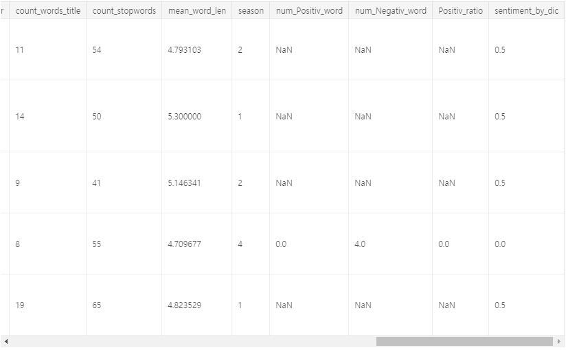
우리는 Positiv_ratio = 긍정적 단어 수 / (긍정 단어 수 + 부정 단어 수)를 정의했습니다. 비율이 0.5보다 작 으면 부정으로 분류되고 0.5보다 크면 긍정적으로 분류됩니다. 나머지를 사용하여 긍정적이거나 부정적인 단어가없는 문장을 포함하는 중립으로 분류했습니다.
앞에서 언급했듯이 usefulCount는 조건에 따라 바이어스를 나타내는 문제를 해결하기 위해 usefulCount를 조건별로 정규화했습니다. 그런 다음 세 개의 예측 감정 값을 추가하고 정규화 된 usefulCount를 곱하여 예측 값을 얻을 수 있습니다.
이제 최종 예측값 순서대로 상태별로 약물을 추천 할 수 있습니다.
def userful_count(data):
    grouped = data.groupby(['condition']).size().reset_index(name='user_size')
    data = pd.merge(data,grouped,on='condition',how='left')
    return data
#___________________________________________________________
df_test =  userful_count(df_test)
df_test['usefulCount'] = df_test['usefulCount']/df_test['user_size']


df_test['deep_pred'] = sub_preds_deep
df_test['machine_pred'] = sub_preds

df_test['total_pred'] = (df_test['deep_pred'] + df_test['machine_pred'] + df_test['sentiment_by_dic'])*df_test['usefulCount']


df_test = df_test.groupby(['condition','drugName']).agg({'total_pred' : ['mean']})
df_test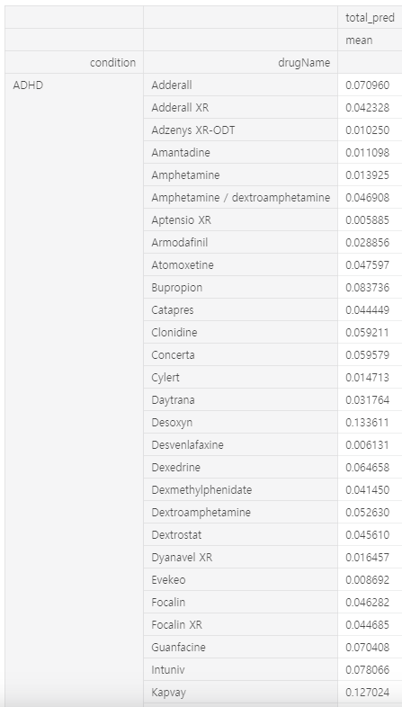
4. 결론 (Conclusion)
- 우리 팀은 환자의 상태에 맞는 의약품을 추천하는 주제를 선정하고 데이터 탐색 - 데이터 전처리 - 모델링을 아우르는 프로젝트를 진행하였습니다.
- 데이터 탐색에서 시각화 기법과 통계기법을 사용하여 데이터의 형식을 살펴보고, 감정을 가장 잘 표현할 수 있는 n-gram과 날짜 및 등급과의 관계등을 찾았습니다.
- 전처리에서는 주제에 맞게 권장하는 약이 하나 뿐인 상태를 제거하고 컴퓨터가 잘 이해할 수 있도록 리뷰들을 전처리 하였습니다.
- 모델링에서는 n-gram을 이용하여 딥러닝을 사용하고, 영화 데이터로 구성된 패키지의 한계를 극복하기 위해 감성 사전을 이용하여 감성분석을 진행하였습니다. 추가적으로 머신러닝모델인 LightGBM을 이용하여 자연어처리의 한계를 극복하려고 시도했습니다.
- 마지막으로 신뢰성 향상을 위해 조건에 따라 유용한 카운트를 정규화 햇습니다. 위의 단계를 통해서 최종 예측 값을 계산하고 값의 순서에 따라 각 조건에 적합한 약물을 추천 할 수 있었습니다.
5. 한계
아래의 내용은 프로젝트동안 저희가 겪은 한게점입니다.
- 감성 사전을 사용한 강성 분석은 양수 단어와 음수 단어 수가 적을때 신뢰도가 적습니다. 예를 들어, 0개의 긍정적인 단어와 1개의 부정적인 단어가 있는 경우, 부정적인 문장으로 분류됩니다. 따라서 감성 단어의 수가 n개 이하이면 관측치를 제외 해야 할 필요가 있습니다.
- 예측값의 신뢰성을 보장하기 위해 유용한 카운트를 정규화하고 예측 값에 곱했습니다. 그러나 누적 사이트 방문자 수가 증가함에 따라 usefulCount는 이전 리뷰에서 더 높은 경향이 있습니다. 따라서 유용한 카운트를 정규화 할때 시간도 함께 고려해야 할 필요가 있습니다.
- 감성이 긍정적이면 신뢰도는 긍정으로 , 감성이 부정이면 신뢰도는 부정으로 향해야 합니다. 그러나 우리는 단순히 유용성에 유용한 카운트를 곱한 것으로 이 부분을 따로 고려하지 않았습니다. 따라서 우리는 서로 다른 감성의 종류에 따라 usefulcount의 부호를 고려하여 곱해야 할 필요가 있습니다.
- 마지막으로, 주제가 의약품과 관련 된 만큼 정확도가 매우 높지 않은 이상은 추천해주는게 위험할 수 있습니다. 비록 온라인으로 소비자가 구매하는 형태이지만 추천이 잘 못 될경우 회사가 잘 못 될 수 있습니다.
'EDA Project > 해외 공모전' 카테고리의 다른 글
| [Kaggle] House Prices: Advanced Regression Techniques (2) (0) | 2020.03.23 |
|---|---|
| [Kaggle] Google Analytics Customer Revenue Prediction (2) | 2018.12.19 |
| [Kaggle] House Prices: Advanced Regression Techniques (0) | 2018.11.27 |


