
| 일 | 월 | 화 | 수 | 목 | 금 | 토 |
|---|---|---|---|---|---|---|
| 1 | 2 | 3 | ||||
| 4 | 5 | 6 | 7 | 8 | 9 | 10 |
| 11 | 12 | 13 | 14 | 15 | 16 | 17 |
| 18 | 19 | 20 | 21 | 22 | 23 | 24 |
| 25 | 26 | 27 | 28 | 29 | 30 | 31 |
- MySQL
- 추천시스템
- TEAM EDA
- 엘리스
- 나는리뷰어다
- 튜토리얼
- 알고리즘
- 프로그래머스
- pytorch
- Object Detection
- 3줄 논문
- 협업필터링
- hackerrank
- Image Segmentation
- TEAM-EDA
- 코딩테스트
- DFS
- 나는 리뷰어다
- Recsys-KR
- 한빛미디어
- 스택
- Segmentation
- Machine Learning Advanced
- 파이썬
- eda
- DilatedNet
- 입문
- Semantic Segmentation
- 큐
- Python
- Today
- Total
TEAM EDA
[Kaggle] House Prices: Advanced Regression Techniques (2) 본문
이번 자료는 지난 자료 House Prices: Advanced Regression Techniques(https://eda-ai-lab.tistory.com/8?category=765157)에 이어서 부족한 부분을 보충해보도록 하겠습니다.
목차
- 결측치 처리
- 변수 탐색
- 모델 해석
1. 결측치 처리
이 대회를 하면서 핵심 중 하나는 데이터의 많은 결측치를 처리하는 부분이었습니다. 이를 해결하기 위해서 결측치가 어떤 식으로 분포해 있고, 어떤 식으로 해결할지에 대해서 분석해보도록 하겠습니다.

81개의 변수 중 40% 정도인 34개의 변수가 결측치를 가지고 있고 몇몇 변수의 경우는 결측치의 비율이 75%가 넘어갑니다. 특징적인 부분으로는 결측치의 비율이 같은 변수들이 있는데,
- 5.44% : GarageFinish, GarageQual, GarageCond, GarageYrBlt, GarageType
- 2.80% : BsmtExposure, BsmtCond, BsmtQual, BsmtFinType2, BsmtFinType1
- 0.82% : MasVnrType, MasVnrArea
- 0.06% : BsmtFullBath, BsmtHalfBath, Functional, Utilities
- 0.03% : GarageArea, GarageCars, Electrical, KitchenQual, TotalBsmtSF, BsmtUnfSF, BsmtFinSF2, BsmtFinSF1, Exterior2nd, Exterior1st, SaleType
- Etc : PoolQC, MiscFeature, Alley, Fence, FireplaceQu, LotFrontage
1.1 Garage Missing Value

출처 : http://officen.kr/wegood/viewcontent.do?id=131&contentID=1879&tab=company&boardType=story
먼저 결측치의 비율이 5.44%인 첫번째 그룹부터 살펴보도록 하겠습니다. 첫 번째 그룹의 각 변수는 주차장과 관련된 변수입니다. 결측치가 발생 가능 한 이유는 아래와 같은데,
- MCAR(Missing completely at Random) : 완전 무작위 결측
- MAR(Missing at Random) : 무작위 결측
- MNAR(Missing at not Random) : 비무작위 결측
데이터의 결측치의 비율이 같은 것을 봐서는 무작위적으로 결측한 것 같지는 않습니다. 합리적인 이유 중 하나는 "주차장이 존재하지 않아서 결측치일 것이다"입니다. 실제로 data_description.txt에도 NA는 No Garage를 의미하고 아래의 GarageArea의 크기가 대부분 0인 것을 통해 확인할 수 있습니다.
total[(total['GarageCars'].notnull()) & (total['GarageFinish'].isnull())][['GarageFinish', 'GarageQual', 'GarageCond', 'GarageYrBlt', 'GarageType', 'GarageCars', 'GarageArea']]['GarageArea'].describe()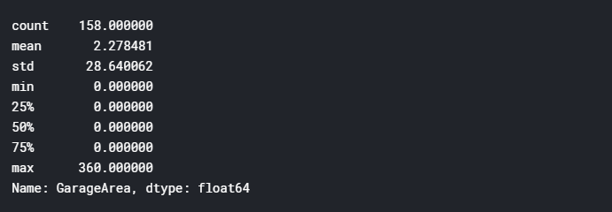
그런데, No Garage인데 GarageArea가 0이 아닌 값이 존재한다는 게 이상합니다. 실제로 아래의 Garage에 대한 결측치 내역을 보면 GarageType만 개수가 2개가 더 적은 것을 볼 수 있습니다.
agg[agg['column'].isin(['GarageFinish', 'GarageQual', 'GarageCond', 'GarageYrBlt', 'GarageType'])]
total[(total['GarageType'].notnull()) & (total['GarageFinish'].isnull())][['GarageFinish', 'GarageQual', 'GarageCond', 'GarageYrBlt', 'GarageType', 'GarageCars', 'GarageArea']]
- 2126번째 index의 경우 주차장은 존재하지만 Garage의 정보가 없는 경우
- 2576의 경우는 애초에 Garage가 없는 것으로 추정
1116의 경우는 GarageType를 NaN으로 바꿈으로서 해결할 수 있습니다. 하지만 666번째 경우는 합리적인 추정을 통해 채워 넣을 수밖에 없습니다. 이를 채워 넣기 위해 동일한 지역에서 GarageCars와 GarageArea가 비슷한 다른 House를 통해 채워 넣도록 하겠습니다.
- Neighborhood(지역), MSZoning(건물 형태), OverallQual(건물 품질), GarageType, GarageCars, GarageArea(크기)
- GarageCars는 1이고 GarageArea는 360과 비슷한 250~450의 값만을 사용하도록 하겠습니다.
- 위를 통해서 결측치가 채워지지 않는 경우 중요도순으로 앞쪽에 있는 변수부터 하나씩 제거해가면서 채우도록 하겠습니다.
- Neighborhood(지역), MSZoning(건물 형태), OverallQual(건물 품질), GarageType, GarageCars, GarageArea(크기)
- MSZoning(건물 형태), OverallQual(건물 품질), GarageType, GarageCars, GarageArea(크기)
- OverallQual(건물 품질), GarageType, GarageCars, GarageArea(크기)
total[(total['Neighborhood'] == 'NAmes') & (total['MSZoning'] == 'RL') & (total['OverallQual'] == 6) & (total['GarageType'] == 'Detchd') & (total['GarageCars'] == 1) & (total['GarageArea'] >= 250) & (total['GarageArea'] <= 450)][['GarageFinish', 'GarageQual', 'GarageType', 'GarageCond', 'GarageYrBlt']]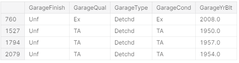
# 참고로 index는 0부터 시작하기에 index 666는 Id 667을 의미합니다.
total.loc[2126, 'GarageFinish'] = 'Unf'
total.loc[2126, 'GarageQual'] = 'TA'
total.loc[2126, 'GarageCond'] = 'TA'
total.loc[2126, 'GarageYrBlt'] = total[(total['Neighborhood'] == 'NAmes') & (total['MSZoning'] == 'RL') & (total['OverallQual'] == 6) & (total['GarageType'] == 'Detchd') & (total['GarageCars'] == 1) & (total['GarageArea'] >= 250) & (total['GarageArea'] <= 450)][['GarageFinish', 'GarageQual', 'GarageType', 'GarageCond', 'GarageYrBlt']]['GarageYrBlt'].median()

total.loc[2576, 'GarageType'] = np.NaN
그 외의 경우는 모두 Garage가 없는 경우로 판단하고 Categorical 변수에는 None을 Numerical 변수에는 -1을 채워 넣도록 하겠습니다.
index = total[total['GarageType'].isnull()].index
for col in ['GarageFinish', 'GarageQual', 'GarageType', 'GarageCond', 'GarageYrBlt']:
    if total[col].dtypes == 'O':
        total.loc[index, col] = 'None'
    else:
        total.loc[index, col] = -1
1.2 Bsmt Missing Value
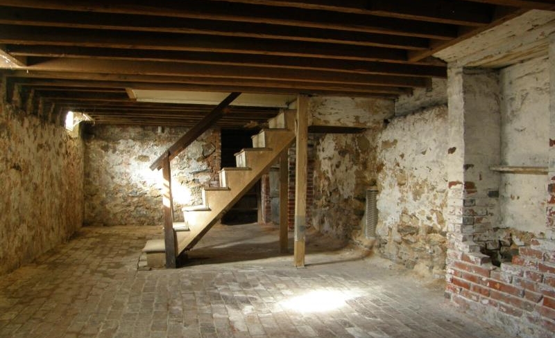
출처 : https://www.thehouseshop.com/property-blog/going-down-under-basement-conversions/18666/
다음으로는 Bsmt와 관련된 결측치들에 대해 살펴보도록 하겠습니다. Bsmt는 basement를 의미하는 것으로 지하실을 의미합니다. basement도 Garage와 마찬가지로 결측치는 지하실이 없는 것을 의미합니다. Garage처럼 특이하게도 지하실이 없지만 다른 값들이 존재하는 경우가 있습니다.
- 2.80% : BstmtExposure, BsmtCond, BsmtQual, BsmtFinType2, BsmtFinType1
agg[agg['column'].isin(['BsmtExposure', 'BsmtCond', 'BsmtQual', 'BsmtFinType2', 'BsmtFinType1'])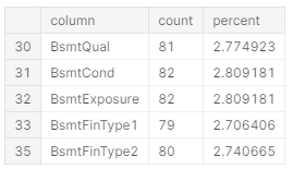
BsmtUnfSF(지하실의 크기)를 의미하는 값이 0이 아니라는 것은 지하실이 있다는 의미입니다. 이를 두 가지 경우로 나누어서 BsmtUnfSF가 있는 경우와 그렇지 않은 경우에 대해 살펴보도록 하겠습니다. 먼저 지하실의 크기가 있는 경우입니다.
total[(total['BsmtUnfSF'].notnull()) & (total['BsmtUnfSF'] != 0) & (total['BsmtExposure'].isnull())][['Neighborhood', 'BsmtExposure', 'BsmtCond', 'BsmtQual', 'BsmtFinType2', 'BsmtFinType1', 'BsmtUnfSF']]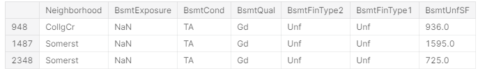
for i in [948, 1487, 2348]:
    A = total.loc[i]
    total.loc[i, 'BsmtExposure'] = total[(total['Neighborhood'] == A['Neighborhood']) & (total['MSZoning'] == A['MSZoning']) & (total['OverallQual'].isin([A['OverallQual']-1, A['OverallQual'], A['OverallQual']+1])) & (total['BsmtCond'] == 'TA') & (total['BsmtQual'] == 'Gd') & (total['BsmtFinType2'] == 'Unf') & (total['BsmtFinType1'] == 'Unf') & (total['BsmtUnfSF'] >= A['BsmtUnfSF']-125) & (total['BsmtUnfSF'] <= A['BsmtUnfSF']+125)]['BsmtExposure'].mode()[0]

    # 결측치가 채워진지 확인
    print("Fill {} Missing Values:".format(i), total.loc[i, 'BsmtExposure'])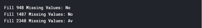
total[(total['BsmtUnfSF'].notnull()) &(total['BsmtUnfSF'] != 0) & (total['BsmtCond'].isnull()) & (total['BsmtQual'].notnull())][['Neighborhood', 'BsmtExposure', 'BsmtCond', 'BsmtQual', 'BsmtFinType2', 'BsmtFinType1', 'BsmtUnfSF']]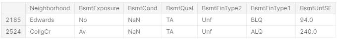
for i in [2185, 2524]:
    A = total.loc[i]
    try:
        total.loc[i, 'BsmtCond'] = total[(total['Neighborhood'] == A['Neighborhood']) & (total['MSZoning'] == A['MSZoning']) & (total['OverallQual'].isin([A['OverallQual']-1, A['OverallQual'], A['OverallQual']+1])) & (total['BsmtExposure'] == A['BsmtExposure']) & (total['BsmtQual'] == A['BsmtQual']) & (total['BsmtFinType2'] == A['BsmtFinType2']) & (total['BsmtFinType1'] == A['BsmtFinType1']) & (total['BsmtUnfSF'] >= A['BsmtUnfSF']-250) & (total['BsmtUnfSF'] <= A['BsmtUnfSF']+250)]['BsmtCond'].mode()[0]

        # 결측치가 채워진지 확인
        print("Fill {} Missing Values:".format(i), total.loc[i, 'BsmtCond'])
    except:
        try:
            total.loc[i, 'BsmtCond'] = total[(total['OverallQual'].isin([A['OverallQual']-1, A['OverallQual'], A['OverallQual']+1])) & (total['BsmtExposure'] == A['BsmtExposure']) & (total['BsmtQual'] == A['BsmtQual']) & (total['BsmtFinType2'] == A['BsmtFinType2']) & (total['BsmtFinType1'] == A['BsmtFinType1']) & (total['BsmtUnfSF'] >= A['BsmtUnfSF']-250) & (total['BsmtUnfSF'] <= A['BsmtUnfSF']+250)]['BsmtCond'].mode()[0]

            # 결측치가 채워진지 확인
            print("Fill {} Missing Values:".format(i), total.loc[i, 'BsmtCond'])
        except:
            print("No Imputation")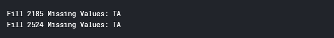
total[(total['BsmtUnfSF'].notnull()) &(total['BsmtUnfSF'] != 0)
& (total['BsmtFinType2'].isnull()) & (total['BsmtQual'].notnull())][['Neighborhood', 'BsmtExposure', 'BsmtCond', 'BsmtQual', 'BsmtFinType2', 'BsmtFinType1', 'BsmtUnfSF']]
for i in [332]:
    A = total.loc[i]
    try:
        total.loc[i, 'BsmtFinType2'] = total[(total['Neighborhood'] == A['Neighborhood']) & (total['MSZoning'] == A['MSZoning']) & (total['OverallQual'].isin([A['OverallQual']-1, A['OverallQual'], A['OverallQual']+1])) & (total['BsmtExposure'] == A['BsmtExposure']) & (total['BsmtQual'] == A['BsmtQual']) & (total['BsmtQual'] == A['BsmtQual']) & (total['BsmtFinType1'] == A['BsmtFinType1']) & (total['BsmtUnfSF'] >= A['BsmtUnfSF']-250) & (total['BsmtUnfSF'] <= A['BsmtUnfSF']+250)]['BsmtFinType2'].mode()[0]

        # 결측치가 채워진지 확인
        print("Fill {} Missing Values:".format(i), total.loc[i, 'BsmtFinType2'])
    except:
        try:
            total.loc[i, 'BsmtFinType2'] = total[(total['OverallQual'].isin([A['OverallQual']-1, A['OverallQual'], A['OverallQual']+1])) & (total['BsmtExposure'] == A['BsmtExposure']) & (total['BsmtQual'] == A['BsmtQual']) & (total['BsmtQual'] == A['BsmtQual']) & (total['BsmtFinType1'] == A['BsmtFinType1']) & (total['BsmtUnfSF'] >= A['BsmtUnfSF']-250) & (total['BsmtUnfSF'] <= A['BsmtUnfSF']+250)]['BsmtFinType2'].mode()[0]

            # 결측치가 채워진지 확인
            print("Fill {} Missing Values:".format(i), total.loc[i, 'BsmtFinType2'])
        except:
            print("No Imputation")
total[(total['BsmtUnfSF'].notnull()) &(total['BsmtUnfSF'] != 0) & (total['BsmtQual'].isnull()) & (total['BsmtFinType2'].notnull())][['Neighborhood', 'BsmtExposure', 'BsmtCond', 'BsmtQual', 'BsmtFinType2', 'BsmtFinType1', 'BsmtUnfSF']]
for i in [2217, 2218]:
    A = total.loc[i]
    try:
        total.loc[i, 'BsmtQual'] = total[(total['Neighborhood'] == A['Neighborhood']) & (total['MSZoning'] == A['MSZoning']) & (total['OverallQual'].isin([A['OverallQual']-1, A['OverallQual'], A['OverallQual']+1])) & (total['BsmtExposure'] == A['BsmtExposure']) & (total['BsmtCond'] == A['BsmtCond']) & (total['BsmtFinType2'] == A['BsmtFinType2']) & (total['BsmtFinType1'] == A['BsmtFinType1']) & (total['BsmtUnfSF'] >= A['BsmtUnfSF']-250) & (total['BsmtUnfSF'] <= A['BsmtUnfSF']+250)]['BsmtQual'].mode()[0]

        # 결측치가 채워진지 확인
        print("Fill {} Missing Values:".format(i), total.loc[i, 'BsmtFinType2'])
    except:
        try:
            total.loc[i, 'BsmtQual'] = total[(total['OverallQual'].isin([A['OverallQual']-1, A['OverallQual'], A['OverallQual']+1])) & (total['BsmtExposure'] == A['BsmtExposure']) & (total['BsmtCond'] == A['BsmtCond']) & (total['BsmtFinType2'] == A['BsmtFinType2']) & (total['BsmtFinType1'] == A['BsmtFinType1']) & (total['BsmtUnfSF'] >= A['BsmtUnfSF']-250) & (total['BsmtUnfSF'] <= A['BsmtUnfSF']+250)]['BsmtQual'].mode()[0]

            # 결측치가 채워진지 확인
            print("Fill {} Missing Values:".format(i), total.loc[i, 'BsmtQual'])
        except:
            print("No Imputation")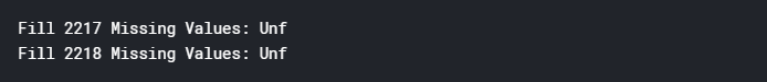
다른 변수들은 모두 지하철의 크기가 있었습니다. 하지만, BsmtCond 같은 경우는 지하실의 크기가 없습니다. 이 값은 다른 정보들을 토대로 BsmtUnfSF값부터 채워 넣고 BsmtCond를 채워 넣도록 하겠습니다.
total[(total['BsmtCond'].isnull()) & (total['BsmtFinType2'].notnull())][['Neighborhood', 'BsmtExposure', 'BsmtCond', 'BsmtQual', 'BsmtFinType2', 'BsmtFinType1', 'BsmtUnfSF']]
for i in [2040]:
    A = total.loc[i]
    total.loc[i, 'BsmtUnfSF'] = total[(total['OverallQual'].isin([A['OverallQual']-1, A['OverallQual'], A['OverallQual']+1])) & (total['BsmtExposure'] == A['BsmtExposure']) & (total['BsmtQual'] == A['BsmtQual']) & (total['BsmtFinType2'] == A['BsmtFinType2']) & (total['BsmtFinType1'] == A['BsmtFinType1'])]['BsmtUnfSF'].median()
    total.loc[i, 'BsmtCond'] = total[(total['OverallQual'].isin([A['OverallQual']-1, A['OverallQual'], A['OverallQual']+1])) & (total['BsmtExposure'] == A['BsmtExposure']) & (total['BsmtQual'] == A['BsmtQual']) & (total['BsmtFinType2'] == A['BsmtFinType2']) & (total['BsmtFinType1'] == A['BsmtFinType1']) & (total['BsmtUnfSF'] >= A['BsmtUnfSF']-250) & (total['BsmtUnfSF'] <= A['BsmtUnfSF']+250)]['BsmtCond'].mode()[0]
    # 결측치가 채워진지 확인
    print("Fill {} Missing Values:".format(i), total.loc[i, 'BsmtCond'])
index = total[total['BsmtQual'].isnull()].index
for col in ['BsmtExposure', 'BsmtCond', 'BsmtQual', 'BsmtFinType2', 'BsmtFinType1']:
    if total[col].dtypes == 'O':
        total.loc[index, col] = 'None'
    else:
        total.loc[index, col] = -1
1.3 MasVnr
다음으로는 MasVnr과 관련된 결측치들에 대해 살펴보도록 하겠습니다. MasVnr는 Masonry veneer의 줄임말로써 Masonry veneer walls consist of a single non-structural external layer of masonry, typically made of brick, stone or manufactured stone이라고 합니다.

MasVnr의 경우 결측치의 경우 None이라는 값을 가집니다.
- 0.82% : MasVnrType, MasVnrArea
agg[agg['column'].isin(['MasVnrType', 'MasVnrArea'])]
print("2 of Variables Missing :", total[(total['MasVnrType'].isnull()) & (total['MasVnrArea'].isnull())][['MasVnrType', 'MasVnrArea']].shape[0])
print("1 of Variables Missing :", total[(total['MasVnrType'].isnull()) & (total['MasVnrArea'].notnull())][['MasVnrType', 'MasVnrArea']].shape[0] +
                                total[(total['MasVnrType'].notnull()) & (total['MasVnrArea'].isnull())][['MasVnrType', 'MasVnrArea']].shape[0])
이제부터는 결측치를 채울 때 선택이 필요합니다. MasVnrType과 MasVnrArea가 모두 없다는 것은 실제로 Masonry veneer가 None일 수도 있고 그렇지 않을 수도 있습니다. MasVnrType이 결측치인 것의 동일한 점이라고는
- Categorical : Street이 Pave, Utilities가 AllPub, LandSlope가 Gtl, Condition2가 Norm, RoofMatl가 Compshg, ExterCond가 TA, Heating이 GasA, Electrical가 SBrkr, PoolQC가 결측치, Fence가 결측치, MiscFeature가 결측치
- Numerical : PoolArea가 0, MiscVal이 0, LowQualFinSF이 0, BsmtHalfBath가 0, 3SsnPorch가 0, ScreenPorch가 0인 정도가 있습니다.
total[total['MiscFeature'].isnull()]['MasVnrType']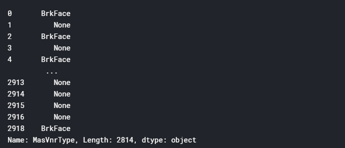
하지만, Masorny veneer가 None인 값들과 섞여있어서 위의 정보만으로는 판단을 내릴 수가 없습니다. 저는 MasVnrArea도 결측치인 경우는 둘 다 None로 채우고, 그렇지 않은 경우는 지역과 Quality, 외벽의 자재를 의미하는 Exterior1st을 통해서 채워 넣도록 하겠습니다.
index = (total['MasVnrType'].isnull()) & (total['MasVnrArea'].isnull())
total.loc[index, 'MasVnrType'] = 'None'
total.loc[index, 'MasVnrArea'] = 0
total[(total['MasVnrType'].isnull()) & (total['MasVnrArea'].notnull())]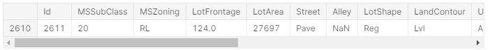
A = total.loc[2610]
total.loc[2610, 'MasVnrType'] = total[(total['Neighborhood'] == A['Neighborhood']) & (total['MSZoning'] == A['MSZoning']) & (total['OverallQual'].isin([A['OverallQual']-1, A['OverallQual'], A['OverallQual']+1])) & (total['Exterior1st'] == A['Exterior1st'])]['MasVnrType'].mode()[0]
1.4 Bsmt and Others
- BsmtFullBath, BsmtHalfBath, Functional, Utilities
agg[agg['column'].isin(['BsmtFullBath', 'BsmtHalfBath', 'Functional', 'Utilities'])]
total[total['BsmtFullBath'].isnull()][['BsmtFullBath', 'BsmtHalfBath', 'Functional', 'Utilities']]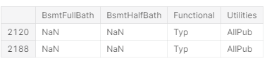
total[total['Functional'].isnull()][['BsmtFullBath', 'BsmtHalfBath', 'Functional', 'Utilities']]
위의 4가지 변수는 결측치의 개수는 2개로 같지만 Basement변수끼리는 연관이 있지만, 다른 두 변수는 다른 변수들과 관련이 없는 것을 볼 수 있습니다.
total[total['BsmtFullBath'].isnull()][['BsmtExposure', 'BsmtCond', 'BsmtQual', 'BsmtFinType2', 'BsmtFinType1','BsmtFullBath','BsmtHalfBath', 'BsmtUnfSF']]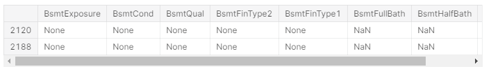
BsmtFullBath, BsmtHalfBath의 경우 지하실이 없는 것으로 보이고 모두 None과 0으로 채워 넣도록 하겠습니다.
index = total['BsmtFullBath'].isnull()
total.loc[index, 'BsmtFullBath'] = 0
total.loc[index, 'BsmtFullBath'] = 0
total.loc[index, 'BsmtUnfSF'] = 0
Functional의 경우 Home functionality (Assume typical unless deductions are warranted)을 의미하는데, 다른 변수들과 연관이 없어서 의미를 통해서 채워 넣기는 힘들어 보입니다. 그래서 동일한 지역의 동일한 가치의 House로 채워 넣도록 하겠습니다.
index = total[total['Functional'].isnull()].index
for i in index:
    A = total.loc[i]
    agg = total[(total['Neighborhood'] == A['Neighborhood']) & (total['OverallQual'].isin([A['OverallQual']-1,A['OverallQual'], A['OverallQual']+1]))]
    total.loc[i, 'Functional'] = agg['Functional'].mode()[0]
    print("Fill {} Missing Values:".format(i), total.loc[i, 'Functional'])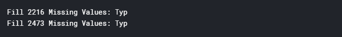
Utilities는 아래와 같으며 전기와 가스, 수도에 따라 순위형을 가지는 가치를 가집니다. 이와 비슷한 변수로는 'Electrical', 'Heating'가 있고 지역, 전기, 가스를 통해서 결측치를 채우도록 하겠습니다.
- AllPub : All public Utilities (E, G, W,& S)
- NoSewr : Electricity, Gas, and Water (Septic Tank)
- NoSeWa : Electricity and Gas Only
- ELO : Electricity only
total.loc[total['Utilities'].isnull()][['Electrical', 'Heating']]
index = total[total['Utilities'].isnull()].index
for i in index:
    A = total.loc[i]
    agg = total[(total['Electrical'] == A['Electrical']) & (total['Heating'] == A['Heating']) & (total['Neighborhood'] == A['Neighborhood']) & (total['OverallQual'].isin([A['OverallQual']-1,A['OverallQual'], A['OverallQual']+1]))]
    try:
        total.loc[i, 'Utilities'] = agg['Utilities'].mode()[0]
        print("Fill {} Missing Values:".format(i), total.loc[i, 'Utilities'])
    except:
        try:
            agg = total[(total['Electrical'] == A['Electrical']) & (total['Heating'] == A['Heating']) & (total['OverallQual'].isin([A['OverallQual']-1,A['OverallQual'], A['OverallQual']+1]))]
            total.loc[i, 'Utilities'] = agg['Utilities'].mode()[0]
            print("Fill {} Missing Values:".format(i), total.loc[i, 'Utilities'])
        except:
            print("No Imputation {}:".format(i))
1.5 ETC
- 의미를 통해 결측치를 채워 넣는 경우
- GarageArea, GarageCars
- TotalBsmtSF, BsmtFinSF1, BsmtFinSF2, FireplaceQu
- LotFrontage
- 결측치가 None을 의미하는 경우 : PoolQC, MiscFeature, Alley, Fence
- 그 외 : Electrical, KitchenQual, Exterior2nd, Exterior1st, SaleType, MSZoning
GarageArea, GarageCars이 결측치인 경우 다른 Garage정보도 결측치입니다. 그래서 마찬가지로 수치형에서 결측치인 0을 넣도록 하겠습니다.
total[total['GarageArea'].isnull()][['GarageArea', 'GarageCars', 'GarageFinish', 'GarageQual', 'GarageType', 'GarageCond', 'GarageYrBlt']]
total.loc[total['GarageArea'].isnull(), 'GarageArea'] = 0
total.loc[total['GarageCars'].isnull(), 'GarageCars'] = 0
아래의 2120번째 index는 대부분의 값이 결측치인 행입니다. BsmtQual이 None인 것으로 보아 Bsmt관련 모든 값들은 0이거나 없어서 결측치이고, PoolArea가 0이므로 PoolQC도 None, Fireplaces가 0이기에 FireplaceQu도 None입니다.
index = total['TotalBsmtSF'].isnull()
total[index][['BsmtQual', 'TotalBsmtSF', 'BsmtUnfSF', 'BsmtFinSF1', 'BsmtFinSF2', 'PoolArea', 'PoolQC', 'MiscFeature', 'Alley', 'Fireplaces', 'FireplaceQu']]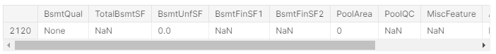
total.loc[index, 'TotalBsmtSF'] = 0
total.loc[index, 'BsmtFinSF1'] = 0
total.loc[index, 'BsmtFinSF2'] = 0
total.loc[index, 'PoolQC'] = 'None'
total.loc[index, 'FireplaceQu'] = 'None'
결측치가 None을 의미하는 경우 : PoolQC, MiscFeature, Alley, Fence
total['PoolQC'] = total['PoolQC'].fillna('None')
total['MiscFeature'] = total['MiscFeature'].fillna('None')
total['Alley'] = total['Alley'].fillna('None')
total['Fence'] = total['Fence'].fillna('None')
FireplaceQu가 결측치인 경우는 Fireplace가 없는 곳으로 Fireplaces 또한 값을 0으로 가집니다.
total[(total['FireplaceQu'].isnull()) & (total['Fireplaces'] != 0)]
total['FireplaceQu'] = total['FireplaceQu'].fillna('None')마찬가지로, BsmtHalfBath가 결측치인 경우는 Basement가 없는 곳으로 BsmtFullBath 또한 값을 0으로 가집니다.
total[total['BsmtHalfBath'].isnull()][['BsmtQual', 'BsmtFullBath', 'BsmtHalfBath']]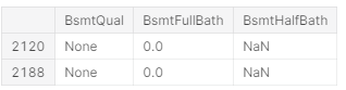
total.loc[total['BsmtHalfBath'].isnull(), 'BsmtHalfBath'] = 0 그 외의 변수는 의미로는 채워 넣기 힘들어서 동일한 지역의 비슷한 조건의 House로 결측치를 채워 넣도록 하겠습니다.
for col in ['Electrical', 'KitchenQual', 'Exterior1st', 'Exterior2nd', 'SaleType']:
    A = total.loc[total[total[col].isnull()].index[0]]
    B = total[(total['Neighborhood'] == A['Neighborhood']) & (total['OverallQual'].isin([A['OverallQual']-1,A['OverallQual'], A['OverallQual']+1]))][col].mode()[0]
    total.loc[total[total[col].isnull()].index[0], col] = B
    print("Fill {} Missing Values:".format(A.Id - 1), B)
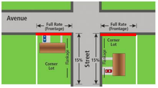
LotFrontage : Linear feet of street connected to property
우리는 LotFrontage가 이웃 간에 집과 유사하다고 가정하여 LotFrontage를 채울 것입니다.
total["LotFrontage"] = total.groupby(["Neighborhood", "OverallQual"])["LotFrontage"].transform(lambda x: x.fillna(x.median()))
total["LotFrontage"] = total.groupby(["Neighborhood"])["LotFrontage"].transform(lambda x: x.fillna(x.median()))
total[total["MSZoning"].isnull()]['Neighborhood']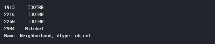
try:
    total["MSZoning"] = total.groupby(["Neighborhood", "OverallQual"])["MSZoning"].transform(lambda x: x.fillna(x.mode()[0]))
except:
    try:
        total["MSZoning"] = total.groupby(["Neighborhood"])["MSZoning"].transform(lambda x: x.fillna(x.mode()[0]))
    except:
        print("No Imputation {}:".format(total[total['MSZoning'].isnull()].index.values))
2. Interactive effectiveness of variables
- 여러 변수의 상호 작용을 분석
- 트리 모델을 통해서 변수의 높은 중요도 확인
- 트리 모델이 학습하는 Node의 관계를 파악
- 그래프를 통한 중요도 파악
- 모델의 잔차와 변수 간의 관계 파악
2.1 여러 변수의 상호작용을 분석
2.1.1 트리 모델의 변수 중요도 파악
from sklearn import tree
from sklearn.ensemble import RandomForestClassifier

clf = tree.DecisionTreeRegressor(max_depth = 10)
clf = clf.fit(df_train[columns], target)

import seaborn as sns
# plot the sorted dataframe
importance = pd.DataFrame()
importance['Feature'] = columns
importance['Importance'] = clf.feature_importances_
importance = importance.sort_values(by='Importance', ascending=False).reset_index(drop=True)
importance = importance[0:10]

(ggplot(data = importance)
 + geom_bar(aes(x='Feature', y='Importance'), fill = '#49beb7', stat='identity', color='black')
 + scale_x_discrete(limits=importance['Feature'].values) # sorting columns
 + theme_light()
 + labs(title = 'Tree Importance Graph : Gini Importance',
         x = '',
         y = 'GINI Importance')
 + theme(axis_text_x = element_text(angle=80),
         figure_size=(10,6))
)
- Categorical : OverallQual
- Numerical : GrLivArea, SndFlrSF, ㄹ, GaragaCars, BsmtFinSF1, 1stFlrSF, YearBuilt, GarageArea, LotFrontage
from sklearn.tree import export_graphviz
clf = tree.DecisionTreeRegressor(max_depth = 3)
clf = clf.fit(df_train[columns], target)
export_graphviz(clf, out_file='tree_limited.dot',
                feature_names = columns, proportion = False, filled = True)

!dot -Tpng tree_limited.dot -o tree_limited.png -Gdpi=600

from IPython.display import Image

Image(filename = 'tree_limited.png')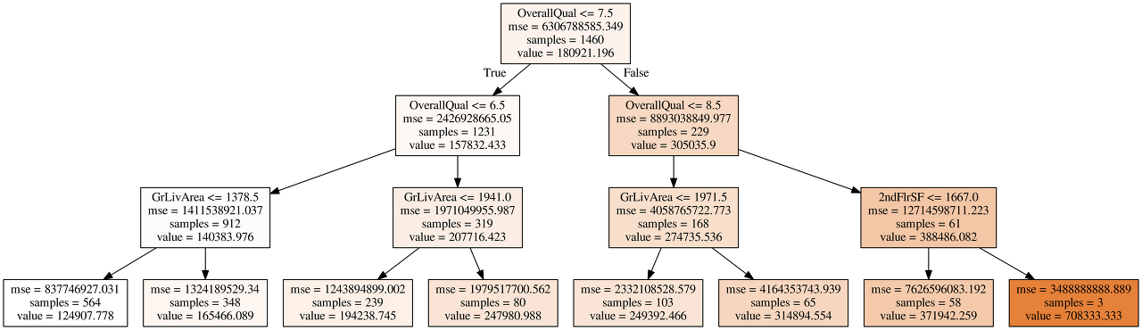
- GrLivArea와 OverallQual
- OverallQual과 2ndFlrSF
2.1.2 그래프를 통한 변수 간의 상호작용 확인
(ggplot(data = df_train)
 + geom_point(aes(x='GrLivArea', y='SalePrice'), stat='identity', color='black', size=0.1)
 + geom_smooth(aes(x='GrLivArea', y='SalePrice'), method='lm', color='#49beb7')
 + facet_wrap('OverallQual')
 + theme_light()
 + labs(title = 'Line Graph of GrLivArea',
         x = 'GrLivArea',
         y = 'SalePrice')
 + theme(axis_text_x = element_text(angle=80),
         figure_size=(10,6))
)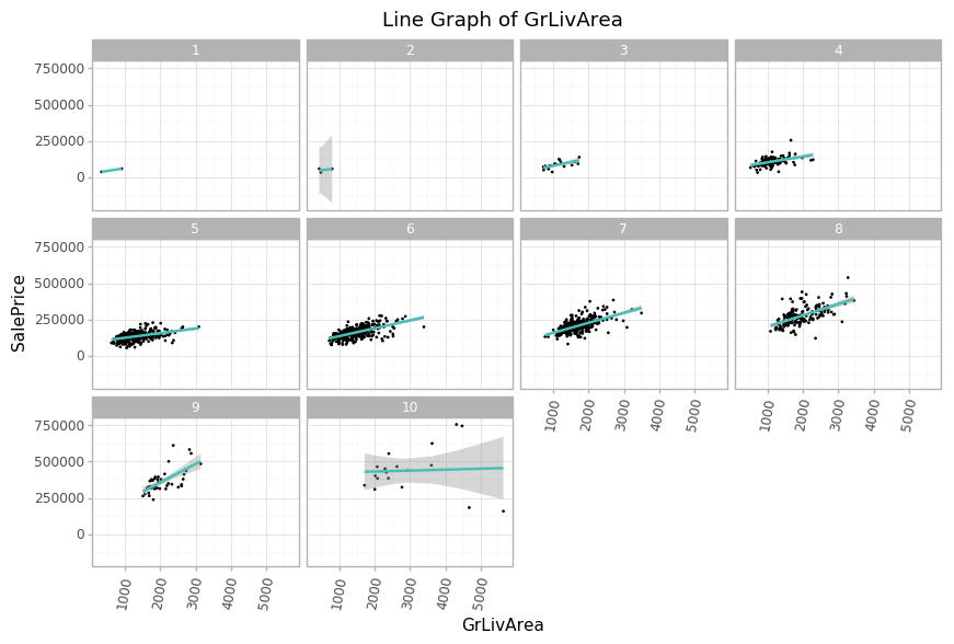
OverallQual이 높아짐에 따라 GrLivArea와 SalePrice 간의 상관관계가 높아지는 것을 볼 수 있습니다. 특이하게 OverallQual이 10인 경우에는 수평의 모습을 보이는데, 두 개의 이상치에 의해 그러한 결과가 나온 것으로 보입니다.
(ggplot(data = df_train)
 + geom_point(aes(x='2ndFlrSF', y='SalePrice'), stat='identity', color='black', size=0.1)
 + geom_smooth(aes(x='2ndFlrSF', y='SalePrice'), color='#49beb7')
 + facet_wrap('OverallQual')
 + theme_light()
 + labs(title = 'Line Graph of 2ndFlrSF',
         x = '2ndFlrSF',
         y = 'SalePrice')
 + theme(axis_text_x = element_text(angle=80),
         figure_size=(10,6))
)
GrLivArea와 마찬가지로 2ndFlrSF도 x와 y 간의 상관관계가 보입니다.
(ggplot(data = df_train)
 + geom_point(aes(x='TotalBsmtSF', y='SalePrice'), stat='identity', color='black', size=0.1)
 + geom_smooth(aes(x='TotalBsmtSF', y='SalePrice'), method='lm', color='#49beb7')
 + facet_wrap('OverallQual')
 + theme_light()
 + labs(title = 'Line Graph of TotalBsmtSF',
         x = 'TotalBsmtSF',
         y = 'SalePrice')
 + theme(axis_text_x = element_text(angle=80),
         figure_size=(10,6))
)
2.2 모델의 잔차와 변수 간의 관계 파악
clf = tree.DecisionTreeRegressor(max_depth = 10)
clf = clf.fit(df_train[columns], target)
oof = clf.predict(df_train[columns])
residual = oof - target

residualDF = pd.DataFrame()
residualDF = pd.concat([residualDF, df_train[columns]], axis=1)
residualDF['residual'] = residual

import scipy as sp

cor_abs = abs(residualDF.corr(method='spearman'))
cor_cols = cor_abs.nlargest(n=10, columns='residual').index # price과 correlation이 높은 column 10개 뽑기(내림차순)

# spearman coefficient matrix
cor = np.array(sp.stats.spearmanr(residualDF[cor_cols].values))[0] # 10 x 10

plt.figure(figsize=(10,10))
sns.set(font_scale=1.25)
sns.heatmap(cor, fmt='.2f', annot=True, square=True , annot_kws={'size' : 8} ,xticklabels=cor_cols.values, yticklabels=cor_cols.values)
잔차와 변수들 간의 상관관계를 살펴보면, 대부분의 값은 0 근처이지만 몇몇 변수는 값이 조금 있습니다. OverallCond 같은 경우를 살펴보면,
df_train['OverallCond'] = df_train['OverallCond'].astype(str)
(ggplot(data = df_train)
 + geom_boxplot(aes(x='OverallCond', y='SalePrice'), color='black', fill='#49beb7')
 # + geom_smooth(aes(x='TotalBsmtSF', y='SalePrice'), method='lm', color='#49beb7')
 + facet_wrap('OverallQual')
 + theme_light()
 + labs(title = 'Boxplot of OverallCond',
         x = 'OverallCond',
         y = 'SalePrice')
 + theme(axis_text_x = element_text(angle=80),
         figure_size=(10,6))
)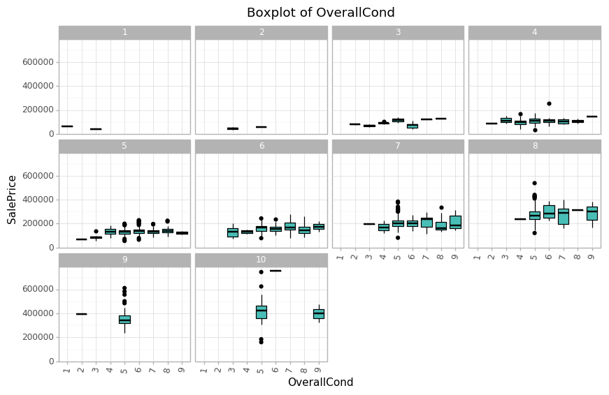
의외로 OverallCond의 경우 OverallQual이 9~10인 경우에 대해 OverallCond가 높지 않은 것을 볼 수 있습니다.
import eli5
import shap

# Explain model predictions using shap library:
explainer = shap.TreeExplainer(clf)
shap_values = explainer.shap_values(df_test[columns])
shap.summary_plot(shap_values, df_test[columns])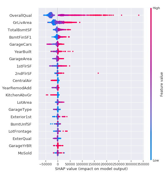
GarageCars의 경우 높은 값을 가져도 중요도가 많이 섞이는 경향이 있어보입니다. 이번 분석을 통해서 변수들에 존재하는 결측치를 채워 넣을 수 있었고 변수들 간의 상호작용과 잔차를 통한 변수의 중요도를 파악하려는 시도를 해봤습니다.
'EDA Project > 해외 공모전' 카테고리의 다른 글
| [kaggle] KUC Hackathon Winter 2018 : What can you do with the Drug Review dataset? (0) | 2020.03.23 |
|---|---|
| [Kaggle] Google Analytics Customer Revenue Prediction (2) | 2018.12.19 |
| [Kaggle] House Prices: Advanced Regression Techniques (0) | 2018.11.27 |


