
Notice
Recent Posts
Recent Comments
Link
| 일 | 월 | 화 | 수 | 목 | 금 | 토 |
|---|---|---|---|---|---|---|
| 1 | 2 | 3 | 4 | 5 | 6 | 7 |
| 8 | 9 | 10 | 11 | 12 | 13 | 14 |
| 15 | 16 | 17 | 18 | 19 | 20 | 21 |
| 22 | 23 | 24 | 25 | 26 | 27 | 28 |
| 29 | 30 | 31 |
Tags
- TEAM EDA
- hackerrank
- 프로그래머스
- DFS
- Image Segmentation
- MySQL
- Object Detection
- 알고리즘
- Semantic Segmentation
- 3줄 논문
- 파이썬
- 스택
- Recsys-KR
- Segmentation
- eda
- 튜토리얼
- 한빛미디어
- 엘리스
- 큐
- TEAM-EDA
- DilatedNet
- 나는 리뷰어다
- Python
- pytorch
- 추천시스템
- Machine Learning Advanced
- 협업필터링
- 입문
- 나는리뷰어다
- 코딩테스트
Archives
- Today
- Total
TEAM EDA
Multi-Scale Context Aggregation by Dilated Convolutions (DilatedNet) Review 본문
EDA Study/Image Segmentation
Multi-Scale Context Aggregation by Dilated Convolutions (DilatedNet) Review
김현우 2021. 2. 6. 19:23Multi-Scale Context Aggregation by Dilated Convolutions (DilatedNet) Review
- papers : https://arxiv.org/pdf/1511.07122.pdf
0. Abstract
- Dense prediction 문제는 일반적으로 Image Classficiation과는 다릅니다.
- Dense prediction 문제에 적합한 새로운 Convolutional Network Module을 제안합니다.
- 제안된 모듈인 Dilated Convolution은 해상도를 잃지 않고 다양한 크기의 contextual information을 통합합니다.
- 특히 Receptive field를 지수적으로 증가시키면서도 해상도를 잃지 않습니다.
- 위의 방법을 통해서 Semantic Segmentation 분야에서 SOTA를 달성할 수 있었습니다.
1. Introduction
- Semantic Segmentation은 다양한 크기의 상황을 추론해야하고 픽셀단위의 분류를 해야하기에 어렵습니다.
- DeconvNet은 위의 문제를 해결하기위해 up-convolutions을 반복해서 다양한 크기의 상황을 추론하고 해상도를 복원했습니다.
- 또 다른 방법은 다양한 크기의 입력을 받아서 이를 결합하는 방식입니다.
- 하지만 이와같은 방법들은 하나의 의문점들을 남기는게 "Down sampling"과 "Rescaled Image"가 필요한지에 대한 의문을 남깁니다.
- DilatedNet에서는 위의 문제를 해결하고자 Down sampling과 Rescaled Image들을 제거합니다.
- 그리고 Dilated라는 Convolution을 여러개 결합해서 Down sampling과 Rescaled Input 없이도 효과적인 결과를 가져옵니다.
2. Dilated Convolutions
- 왼쪽은 일반적은 Convolution을 의미하고 오른쪽은 Dilated Convolution을 의미합니다.
- Convolution과 Dilated Convolution의 가장 큰 차이는 Kernel의 t에 l이라는 값이 붙어있는 점입니다.
- 이 값에 의해서 둘다 동일하게 3x3의 필터를 가지지만 Receptive Field는 3x3과 5x5로 차이가 발생합니다.
위의 수식이 가지는 의미를 한번 예시로 살펴보도록 하겠습니다. 아래의 내용에 있는 수식과 그림은 안성호님의 블로그의 내용의 사진을 참고하였습니다.
여기서 y는 output, x는 input, h는 kernel을 의미합니다. 실제 아래의 예시에 대해서 위의 수식이 어떤 값을 가지는지 확인해보겠습니다.
- output -13은 아래와 같은 과정을 통해서 나오게 됩니다.
- 한번 같은 과정을 Dilated가 2인 경우에 대해서 적용해보겠습니다.
- 위와 같은 Dilated 과정을 통해서 Receptive Field가 넓어지는 과정은 아래와 같습니다.
- (a) : F0 (receptive filed, green) → "3x3 filter with 1-dilated convolution" (parameter 9개, red points) → F1
- (b) : F1 (receptive filed, green)→ "3x3 filter with 2-dilated convolution, padding 1" (parameter 9개, red points) ≒ 7x7 filter → F2
- (c) : F2 (receptive filed, green)→ "3x3 filter with 4-dilated convolution, padding 3" (parameter 9개, red points) ≒ 15 x 15 filter → F3
- Convolution의 경우 파라미터가 갯수가 선형으로 증가하지만, Dilated Convolution은 지수적으로 증가하므로 효율적입니다.
- Fi+1 = 2i+2 -1 * 2i+2 -1 의 Receptive Field를 가집니다.
3. Multi-Scale Context Aggregation
- Context module : multi-scale contextual information을 집계하여 dense prediction 구조의 성능을 높이기 위함입니다.
- input of context module : font-end(e.g. vgg16)를 통해 해상도가 64x64의 feature map 입니다.
- Layer 1 ~ Layer 7 : 3x3 convolution with diffrent dilation 을 사용합니다.
- Layer 8 : 1x1 convolution with 1-dilation 을 사용합니다.
- truncation : colvolution 이후에 activation function을 ReLU 사용합니다.
- Receptive Field의 경우 원본 이미지를 중심으로 계산하기에 Layer1과 2의 경우 Dilation이 1으로 동일해도 크기가 다릅니다. 아래의 그림에서처럼 Layer 2의 경우에 대해서는 이미 원본 이미지를 피쳐맵으로 바꾼 데이터에 대해 적용됩니다.
- 논문에서는 Initialization (Le, Quoc V., Jaitly, Navdeep, and Hinton, Geoffrey E. A simple way to initialize recurrent networks of rectified linear units. arXiv:1504.00941, 2015) 방식을 사용했습니다.
- a : the index of the input feature map
- b : the index of the output map
- 정확한 수식이 의미하는 바는 모르겠지만 아래의 코드를 함께봤을때 이전의 Weight값을 그대로 가져와서 초기화시키지 않은가 생각은 듭니다. (확실하지는 않습니다)
                L.Convolution(
                    prev_layer,
                    param=[dict(lr_mult=1, decay_mult=1),
                           dict(lr_mult=2, decay_mult=0)],
                    convolution_param=dict(
                        num_output=num_classes * multiplier, kernel_size=3,
                        dilation=dilation, pad=dilation,
                        weight_filler=dict(type='identity',
                                           num_groups=num_classes,
                                           std=0.01 / multiplier),
                        bias_filler=dict(type='constant', value=0))))
4. Front END
- a front-end prediction module : VGG-16 네트워크를 사용합니다.
- 마지막 두개의 layer에 존재하는 pooing 및 striding 제거합니다.
- 마지막 layer를 제외한 모든 layer의 convolution 연산은 2-dilated 적용합니다.
- 마지막 layer의 convolution 은 4-dialted 적용합니다.
- convolution을 바꾸면서 기존 학습된 weight를 모두 초기화시켜야 했지만, 고해상도의 output을 얻을 수 있다.
- https://blog.kakaocdn.net/dn/XGBYY/btqV19gdFgI/wxWK9K9pERO4qeaMvTxt11/img.png
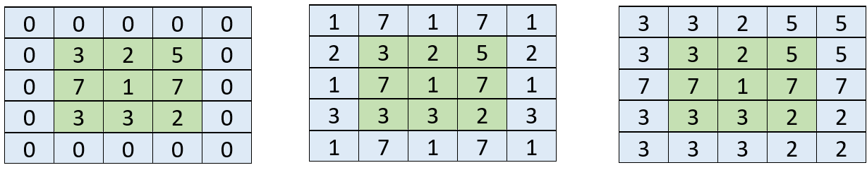
Padding of 1 adds an extra layers on top of the input matrix. Left: Zero padding. Middle: Reflection padding. Right: Replication padding.
Training
- SGD
- minibatch size : 14
- learning rate : 10-3
- momentum : 0.9
- iteration : 60K
Semantic segmentations produced by different adaptations of the VGG-16 classification network.
Our front-end prediction module is simpler and more accurate than prior models. This table reports accuracy on the VOC-2012 test set.
5. Experiments
Semantic segmentations produced by different models.
Controlled evaluation of the effect of the context module on the accuracy of three different architectures for semantic segmentation.
Evaluation on the VOC-2012 test set. ‘DeepLab++’ stands for DeepLab-CRF-COCO-LargeFOV and ‘DeepLab-MSc++’ stands for DeepLab-MSc-CRF-LargeFOV-COCO-CrossJoint (Chen et al., 2015a).
6. Conclusion
참고자료
'EDA Study > Image Segmentation' 카테고리의 다른 글
| A Deep Convolutional Encoder-Decoder Architecture for Image Segmentation (SegNet) (2) | 2021.09.21 |
|---|---|
| Deconvolutional Network (DeconvNet) Code (0) | 2021.09.21 |
| Deconvolutional Network (DeconvNet) (4) | 2021.09.21 |
| Fully Convolutional Networks (FCN) Code (0) | 2021.09.21 |
| Fully Convolutional Networks (FCN) (0) | 2021.09.21 |
'EDA Study/Image Segmentation' Related Articles
more


